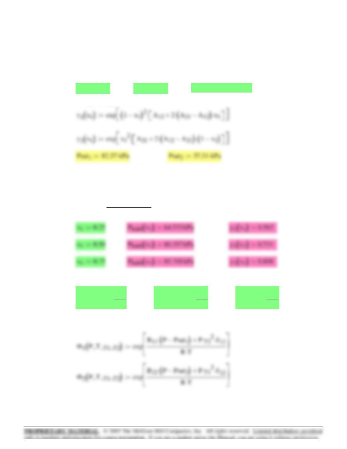
δ12 2B
12
⋅B11
−B22
−:=
B12 52 cm3
mol
⋅:=B22 1523−cm3
mol
⋅:=B11 963−cm3
mol
⋅:=
BUBL P calculations with virial coefficients:(b)
y1x1
()
x1γ1x1
()
⋅Psat1
⋅
Pbubl x1
()
:=
Pbubl x1
()
x1γ1x1
()
⋅Psat1
⋅1x
1
−
()
γ2x1
()
⋅Psat2
⋅+:=
BUBL P calculations based on Eq. (10.5):(a)
Margules equations:
T 55 273.15+()K⋅:=A21 1.42:=A12 0.59:=
14.1
Chapter 14 – Section A – Mathcad Solutions
539
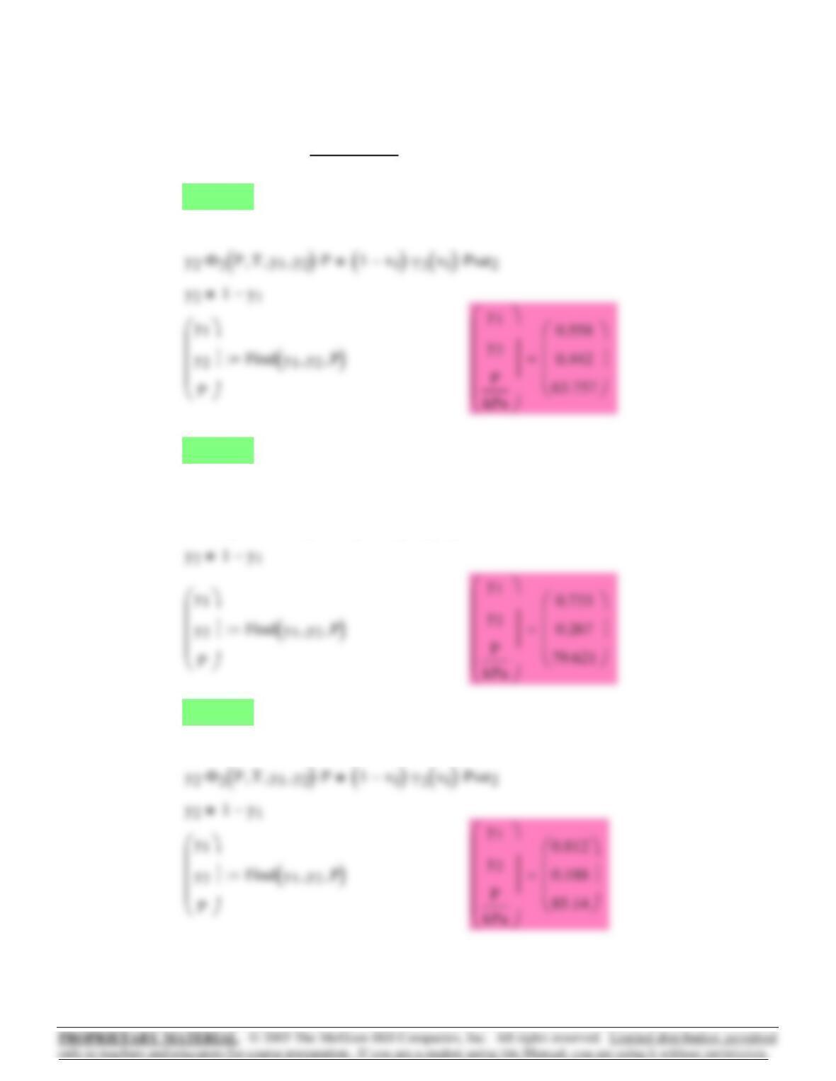
y1Φ1PT,y1
,y2
,
()
⋅P⋅x1γ1x1
()
⋅Psat1
⋅=
Givenx10.75:=
y2Φ2PT,y1
,y2
,
()
⋅P⋅1x
1
−
()
γ2x1
()
⋅Psat2
⋅=
y1Φ1PT,y1
,y2
,
()
⋅P⋅x1γ1x1
()
⋅Psat1
⋅=
Givenx10.50:=
y1Φ1PT,y1
,y2
,
()
⋅P⋅x1γ1x1
()
⋅Psat1
⋅=
Givenx10.25:=
y21y
1
−:=y10.5:=PPsat1Psat2
+
2
:=
Guess:
540
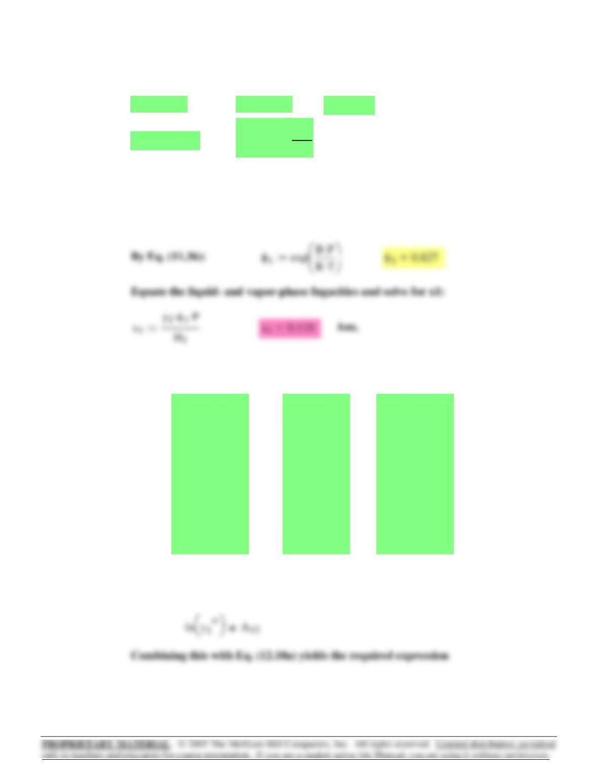
It follows immediately from Eq. (12.10a) that:(a)
Psat2P1
:=x21x
1
−:=i 2 rows P()..:=
y1
0.000
0.2716
0.4565
0.5934
0.6815
0.7440
0.8050
0.8639
⎛
⎜
⎜
⎜
⎜
⎜
⎜
⎜
⎜
⎜
⎜
⎝
⎞
⎟
⎟
⎟
⎟
⎟
⎟
⎟
⎟
⎠
:=
P
12.30
15.51
18.61
21.63
24.01
25.92
27.96
30.12
⎛
⎜
⎜
⎜
⎜
⎜
⎜
⎜
⎜
⎜
⎜
⎝
⎞
⎟
⎟
⎟
⎟
⎟
⎟
⎟
⎟
⎠
:=
x1
0.000
0.0895
0.1981
0.3193
0.4232
0.5119
0.6096
0.7135
⎛
⎜
⎜
⎜
⎜
⎜
⎜
⎜
⎜
⎜
⎜
⎝
⎞
⎟
⎟
⎟
⎟
⎟
⎟
⎟
⎟
⎠
:=
Data:
Pressures in kPa14.4
⎜
fhat1vy1φ1
⋅P⋅=
fhat1lH1x1
⋅=
Assume Henry’s law applies to methane(1) in the liquid phase, and that the
Lewis/Randall rule applies to the methane in the vapor:
B 105−cm3
mol
⋅:=H1200 bar⋅:=
y10.95:=P 30 bar⋅:=T 200 K⋅:=
14.3
541
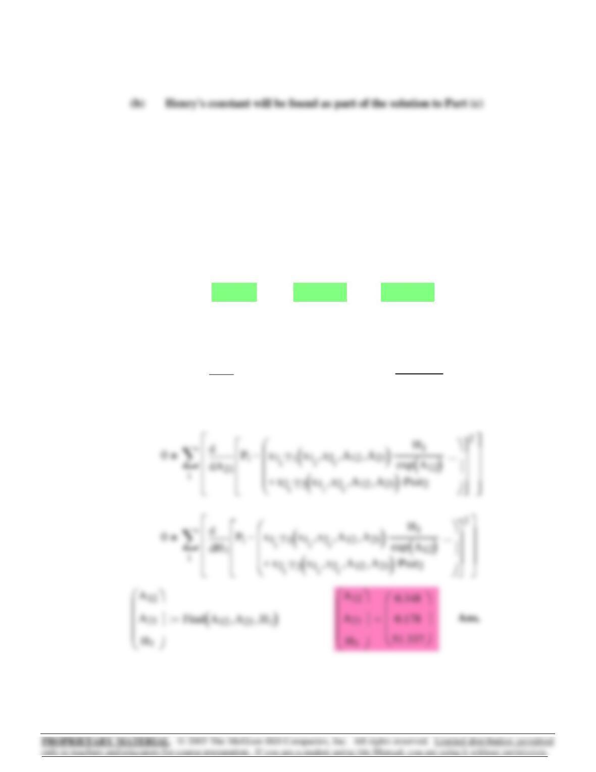
0
iA12
Pix1iγ1x1ix2i
,A12
,A21
,
()
⋅H1
exp A12
()
⋅
x2iγ2x1ix2i
,A12
,A21
,
()
⋅Psat2
⋅+
…
⎛
⎜
⎜
⎜
⎝
⎞
⎟
⎠
−
⎡
⎢
⎢
⎢
⎣
⎤
⎥
⎥
⎥
⎦
2
d
d
⎡
⎢
⎢
⎢
⎣
⎤
⎥
⎥
⎥
⎦
∑
=
Given
Mininize the sums of the squared errors by
setting sums of derivatives equal to zero.
A12 0.4:=A21 0.2:=H150:=
Guesses:
γ2x1 x2,A12
,A21
,
()
exp x1()
2A21 2A
12 A21
−
()
⋅x2⋅+
⎡
⎣
⎤
⎦
⋅
⎡
⎣
⎤
⎦
:=
γ1x1 x2,A12
,A21
,
()
exp x2()
2A12 2A
21 A12
−
()
⋅x1⋅+
⎡
⎣
⎤
⎦
⋅
⎡
⎣
⎤
⎦
:=
The most satisfactory procedure for reduction of this set of data is to find
the value of Henry’s constant by regression along with the Margules
parameters.
BARKER’S METHOD by non-linear least squares.
Margules equation.
(c)
542
⎜
⎜
⎜
⎜
⎜
⎜
⎢
⎢
⎥
⎥
⎢
⎢
⎥
⎥
⎜
⎜
⎢
⎢
⎥
⎥
⎢
⎢
⎥
⎥
(d) γ1x1x2,( ) exp x22A12 2A
21 A12
−
()
⋅x1⋅+
⎡
⎣
⎤
⎦
⋅
⎡
⎣
⎤
⎦
:=
γ2x1x2,( ) exp x12A21 2A
12 A21
−
()
⋅x2⋅+
⎡
⎣
⎤
⎦
⋅
⎡
⎣
⎤
⎦
:=
0.2
y1iy1calci
−
()
100⋅
Fit GE/RT data to Margules eqn. by least squares:
i 2 rows P()..:= y21y
1
−:=
Given
0
iA12
x1iln
y1iPi
⋅
x1i
H1
exp A12
()
⋅
⎛
⎜
⎜
⎜
⎝
⎞
⎟
⎠
⋅
x2iln
y2iPi
⋅
x2iPsat2
⋅
⎛
⎜
⎜
⎝
⎞
⎠
⋅+
…
⎛
⎜
⎜
⎜
⎜
⎜
⎜
⎝
⎞
⎟
⎟
⎟
⎟
⎠
A21 x1i
⋅
A12 x2i
⋅+
…
⎛
⎜
⎜
⎝
⎞
⎠
x1i
⋅x2i
⋅−
⎡
⎢
⎢
⎢
⎢
⎢
⎢
⎣
⎤
⎥
⎥
⎥
⎥
⎥
⎥
⎦
2
d
d
∑
=
543
0
iA21
x1iln
y1iPi
⋅
x1i
H1
exp A12
()
⋅
⎛
⎜
⎜
⎜
⎝
⎞
⎟
⎠
⋅
x2iln
y2iPi
⋅
x2iPsat2
⋅
⎛
⎜
⎜
⎝
⎞
⎠
⋅+
…
⎛
⎜
⎜
⎜
⎜
⎜
⎜
⎝
⎞
⎟
⎟
⎟
⎟
⎠
A21 x1i
⋅
A12 x2i
⋅+
…
⎛
⎜
⎜
⎝
⎞
⎠
x1i
⋅x2i
⋅−
⎡
⎢
⎢
⎢
⎢
⎢
⎢
⎣
⎤
⎥
⎥
⎥
⎥
⎥
⎥
⎦
2
d
d
∑
=
γ1x1x2,( ) exp x22A12 2A
21 A12
−
()
⋅x1⋅+
⎡
⎣
⎤
⎦
⋅
⎡
⎣
⎤
⎦
:=
⎡
⎣
⎤
⎦
⎡
⎣
⎤
⎦
544
⎜
⎜
⎜
⎜
⎜
⎜
⎜
⎜
⎢
⎢
⎥
⎥
⎜
⎜
⎜
⎜
It follows immediately from Eq. (12.10a) that:(a)
Psat1P8
:=x21x
1
−:=i17..:=
y1
0.5934
0.6815
0.7440
0.8050
0.8639
0.9048
0.9590
1.000
⎛
⎜
⎜
⎜
⎜
⎜
⎜
⎜
⎜
⎜
⎜
⎝
⎞
⎟
⎟
⎟
⎟
⎟
⎟
⎟
⎟
⎠
:=
P
21.63
24.01
25.92
27.96
30.12
31.75
34.15
36.09
⎛
⎜
⎜
⎜
⎜
⎜
⎜
⎜
⎜
⎜
⎜
⎝
⎞
⎟
⎟
⎟
⎟
⎟
⎟
⎟
⎟
⎠
:=
x1
0.3193
0.4232
0.5119
0.6096
0.7135
0.7934
0.9102
1.000
⎛
⎜
⎜
⎜
⎜
⎜
⎜
⎜
⎜
⎜
⎜
⎝
⎞
⎟
⎟
⎟
⎟
⎟
⎟
⎟
⎟
⎠
:=
Data:
Pressures in kPa14.5
0 0.2 0.4 0.6 0.8
0.6
0
PiPcalci
−
−
()
x1i
545
γ2x1x2,( ) exp x12A21 2A
12 A21
−
()
⋅x2⋅+
⎡
⎣
⎤
⎦
⋅
⎡
⎣
⎤
⎦
:=
γ1x1x2,( ) exp x22A12 2A
21 A12
−
()
⋅x1⋅+
⎡
⎣
⎤
⎦
⋅
⎡
⎣
⎤
⎦
:=
(d)
0
iA12
Pix1iγ1x1ix2i
,A12
,A21
,
()
⋅Psat1
⋅
x2iγ2x1ix2i
,A12
,A21
,
()
⋅H2
exp A21
()
⋅+
…
⎛
⎜
⎜
⎜
⎝
⎞
⎟
⎠
−
⎡
⎢
⎢
⎢
⎣
⎤
⎥
⎥
⎥
⎦
2
d
d
⎡
⎢
⎢
⎢
⎣
⎤
⎥
⎥
⎥
⎦
∑
=
Given
⎡
⎣
⎤
⎦
⎡
⎣
⎤
⎦
⎡
⎣
⎤
⎦
⎡
⎣
⎤
⎦
The most satisfactory procedure for reduction of this set of data is to find
the value of Henry’s constant by regression along with the Margules
parameters.
BARKER’S METHOD by non-linear least squares.
Margules equation.
(c)
546
⎜
⎜
⎜
⎜
⎜
⎜
⎢
⎢
⎥
⎥
⎢
⎢
⎥
⎥
⎜
⎜
⎢
⎢
⎥
⎥
⎢
⎢
⎥
⎥
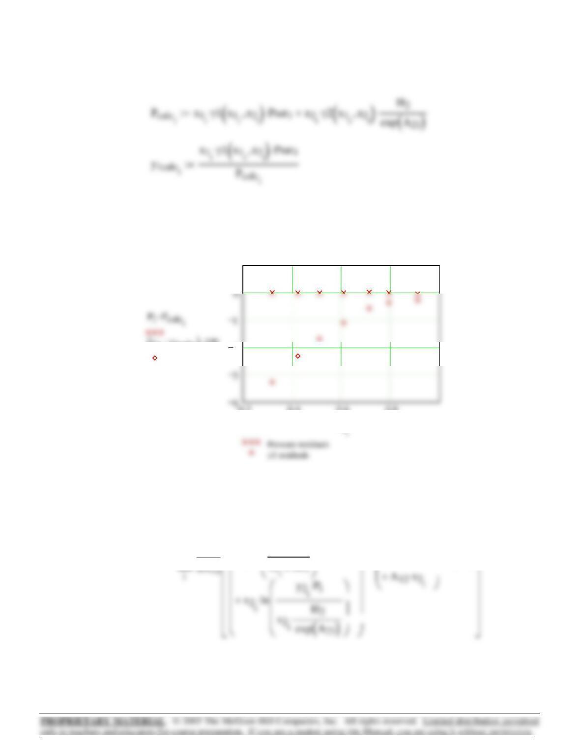
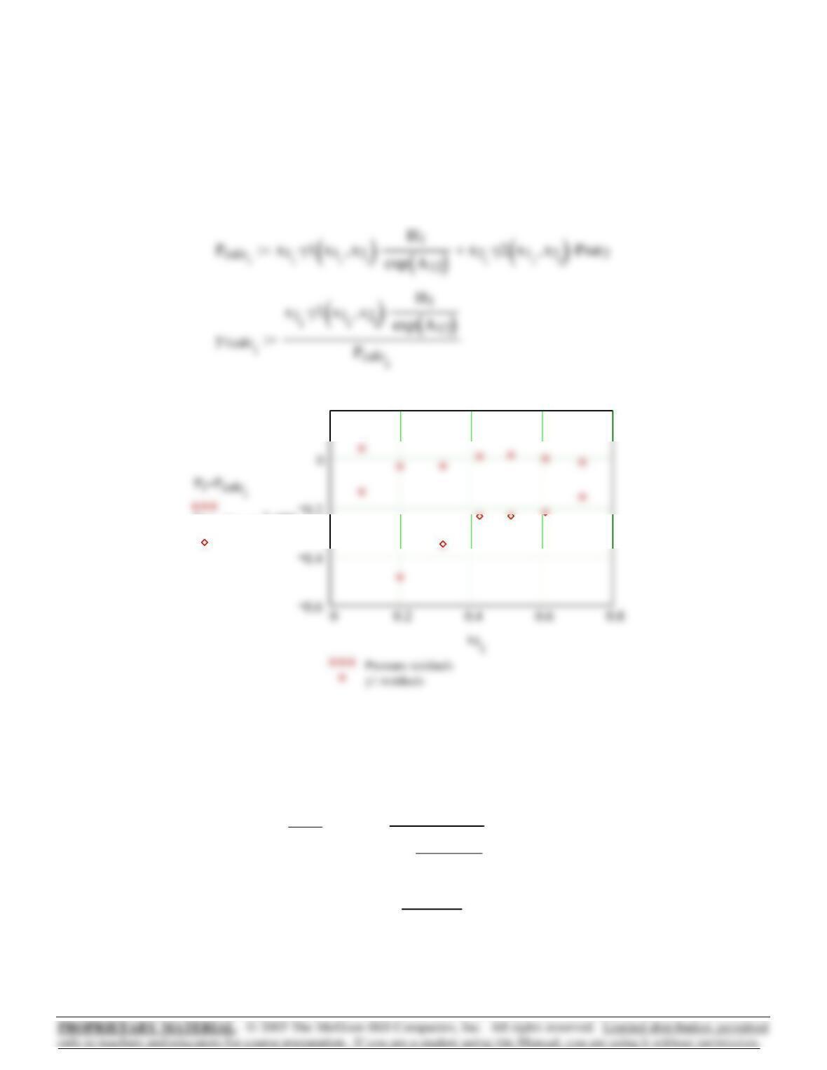
The plot of residuals below shows that the procedure used (Barker’s
method with regression for H2) is not in this case very satisfactory, no
doubt because the data do not extend close enough to x1 = 0.
0.2 0.4 0.6 0.8
2
1
y1iy1calci
−
()
100⋅
x1i
Fit GE/RT data to Margules eqn. by least squares:
i17..:= y21y
1
−:=
Given
0
⎜
x1iln
y1iPi
⋅
x1iPsat1
⋅
⎛
⎜
⎜
⎞
⋅
…
⎛
⎜
⎞
A21 x1i
⋅
…
⎛
⎜
⎞
x1i
⋅x2i
⋅−
⎡
⎢
⎤
⎥
2
d
∑
=
547
0
iA21
x1iln
y1iPi
⋅
x1iPsat1
⋅
⎛
⎜
⎜
⎝
⎞
⎠
⋅
x2iln
y2iPi
⋅
x2i
H2
exp A21
()
⋅
⎛
⎜
⎜
⎜
⎝
⎞
⎟
⎠
⋅+
…
⎛
⎜
⎜
⎜
⎜
⎜
⎜
⎝
⎞
⎟
⎟
⎟
⎟
⎠
A21 x1i
⋅
A12 x2i
⋅+
…
⎛
⎜
⎜
⎝
⎞
⎠
x1i
⋅x2i
⋅−
⎡
⎢
⎢
⎢
⎢
⎢
⎢
⎣
⎤
⎥
⎥
⎥
⎥
⎥
⎥
⎦
2
d
d
∑
=
0
x1iln
y1iPi
⋅
x1iPsat1
⋅
⎛
⎜
⎜
⎞
⋅
…
⎛
⎜
⎞
A21 x1i
⋅
…
⎛
⎜
⎞
x1i
⋅x2i
⋅−
⎡
⎢
⎤
⎥
2
d
d
∑
=
548
⎜
⎜
⎜
⎜
⎢
⎥
⎜
⎜
⎜
⎡
⎤
⎡
⎤
It follows immediately from Eq. (12.10a) that:(a)
Psat2P1
:=x21x
1
−:=i 2 rows P()..:=
y1
0.0
0.1794
0.2383
0.3302
0.3691
0.4628
0.6184
0.7552
0.8378
0.9137
⎛
⎜
⎜
⎜
⎜
⎜
⎜
⎜
⎜
⎜
⎜
⎜
⎜
⎜
⎝
⎞
⎟
⎟
⎟
⎟
⎟
⎟
⎟
⎟
⎟
⎟
⎟
⎠
:=
x1
0.0
0.0932
0.1248
0.1757
0.2000
0.2626
0.3615
0.4750
0.5555
0.6718
⎛
⎜
⎜
⎜
⎜
⎜
⎜
⎜
⎜
⎜
⎜
⎜
⎜
⎜
⎝
⎞
⎟
⎟
⎟
⎟
⎟
⎟
⎟
⎟
⎟
⎟
⎟
⎠
:=
P
15.79
17.51
18.15
19.30
19.89
21.37
24.95
29.82
34.80
42.10
⎛
⎜
⎜
⎜
⎜
⎜
⎜
⎜
⎜
⎜
⎜
⎜
⎜
⎜
⎝
⎞
⎟
⎟
⎟
⎟
⎟
⎟
⎟
⎟
⎟
⎟
⎟
⎠
:=
Data:
Pressures in kPa14.6
0.3 0.4 0.5 0.6 0.7 0.8 0.9 1
0.6
−
()
x1i
549
0
iA12
Pix1iγ1x1ix2i
,A12
,A21
,
()
⋅H1
exp A12
()
⋅
x2iγ2x1ix2i
,A12
,A21
,
()
⋅Psat2
⋅+
…
⎛
⎜
⎜
⎜
⎝
⎞
⎟
⎠
−
⎡
⎢
⎢
⎢
⎣
⎤
⎥
⎥
⎥
⎦
2
d
d
⎡
⎢
⎢
⎢
⎣
⎤
⎥
⎥
⎥
⎦
∑
=
Given
⎡
⎣
⎤
⎦
⎡
⎣
⎤
⎦
γ1x1 x2,A12
,A21
,
()
exp x2()
2A12 2A
21 A12
−
()
⋅x1⋅+
⎡
⎣
⎤
⎦
⋅
⎡
⎣
⎤
⎦
:=
The most satisfactory procedure for reduction of this set of data is to
find the value of Henry’s constant by regression along with the
Margules parameters.
BARKER’S METHOD by non-linear least squares.
Margules equation.
(c)
550
⎜
⎜
⎜
⎜
⎜
⎜
⎢
⎢
⎥
⎥
⎢
⎢
⎥
⎥
⎜
⎜
⎢
⎢
⎥
⎥
⎢
⎢
⎥
⎥
(d) γ1x1x2,( ) exp x22A12 2A
21 A12
−
()
⋅x1⋅+
⎡
⎣
⎤
⎦
⋅
⎡
⎣
⎤
⎦
:=
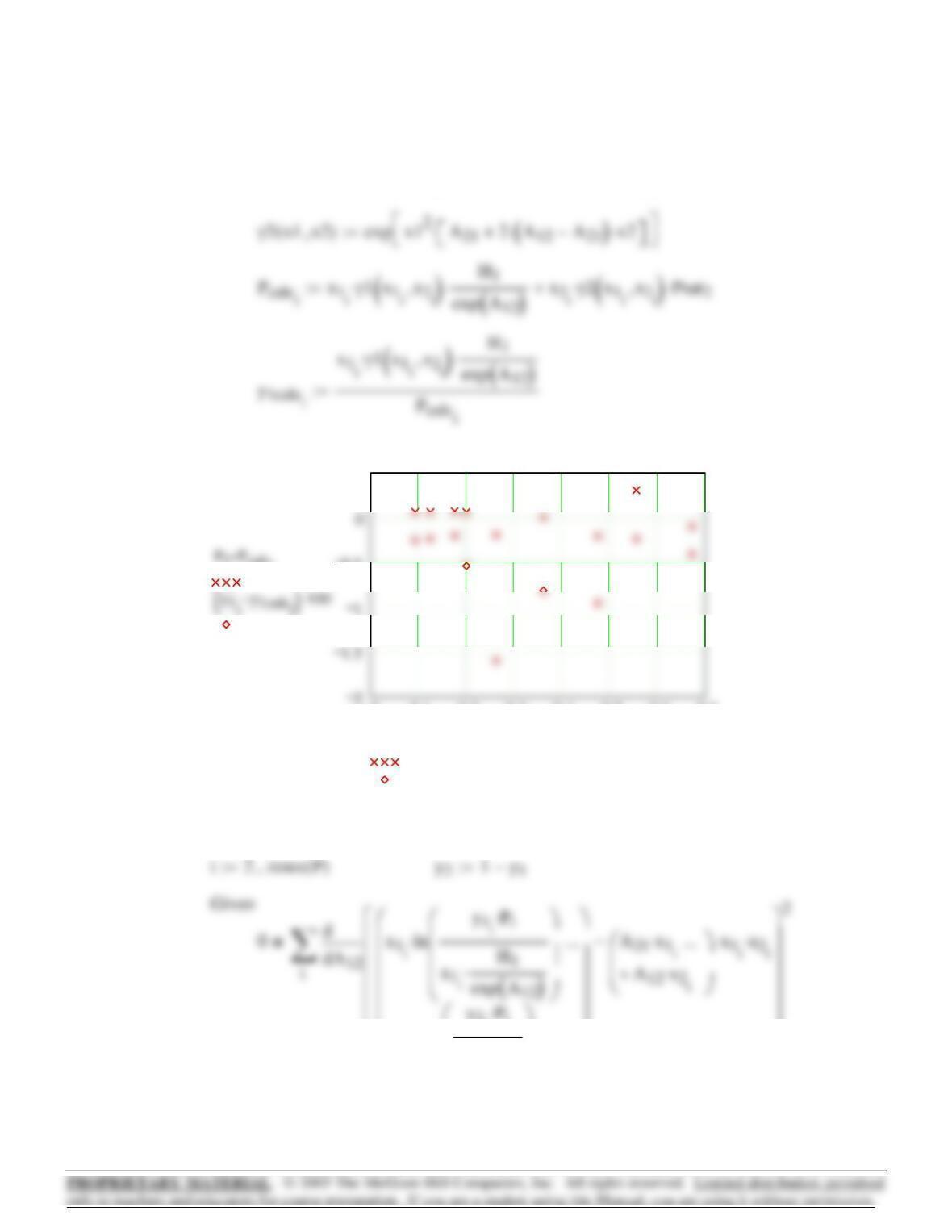
0 0.1 0.2 0.3 0.4 0.5 0.6 0.7
0.5
0.5
Pressure residuals
y1 residuals
x1i
Fit GE/RT data to Margules eqn. by least squares:
⎜
⎜
⎜
⎜
⎢
⎥
x2iln
x2iPsat2
⋅
⎛
⎜
⎜
⎝
⎞
⎠
⋅+
⎜
⎜
⎝
⎟
⎠
⎢
⎢
⎣
⎥
⎥
⎦
551
⎡
⎣
⎤
⎦
⎡
⎣
⎤
⎦
y1iPi
⋅
⎛
⎞
⎛
⎞
⎡
⎤
2
iH1
x1i
H1
exp A12
()
⋅
⎜
⎜
⎝
⎟
⎠
⎜
⎜
⎜
⎜
⎜
y2iPi
⋅
⎜
⎜
⎜
⎟
⎟
⎟
A12 x2i
⋅+
⎛
⎜
⎜
⎝
⎞
⎠
⎢
⎢
⎢
⎥
⎥
⎥
d
∑
γ1x1x2,( ) exp x22A12 2A
21 A12
−
()
⋅x1⋅+
⎡
⎣
⎤
⎦
⋅
⎡
⎣
⎤
⎦
:=
γ2x1x2,( ) exp x12A21 2A
12 A21
−
()
⋅x2⋅+
⎡
⎣
⎤
⎦
⋅
⎡
⎣
⎤
⎦
:=
552
⎜
⎜
⎜
⎜
⎜
⎜
⎢
⎥
⎜
⎜
⎢
⎥
It follows immediately from Eq. (12.10a) that:(a)
Psat1P10
:=x21x
1
−:=i19..:=
y1
0.3302
0.3691
0.4628
0.6184
0.7552
0.8378
0.9137
0.9860
0.9945
1.0000
⎛
⎜
⎜
⎜
⎜
⎜
⎜
⎜
⎜
⎜
⎜
⎜
⎜
⎜
⎝
⎞
⎟
⎟
⎟
⎟
⎟
⎟
⎟
⎟
⎟
⎟
⎟
⎠
:=
P
19.30
19.89
21.37
24.95
29.82
34.80
42.10
60.38
65.39
69.36
⎛
⎜
⎜
⎜
⎜
⎜
⎜
⎜
⎜
⎜
⎜
⎜
⎜
⎜
⎝
⎞
⎟
⎟
⎟
⎟
⎟
⎟
⎟
⎟
⎟
⎟
⎟
⎠
:=
x1
0.1757
0.2000
0.2626
0.3615
0.4750
0.5555
0.6718
0.8780
0.9398
1.0000
⎛
⎜
⎜
⎜
⎜
⎜
⎜
⎜
⎜
⎜
⎜
⎜
⎜
⎜
⎝
⎞
⎟
⎟
⎟
⎟
⎟
⎟
⎟
⎟
⎟
⎟
⎟
⎠
:=
Data:
Pressures in kPa14.7
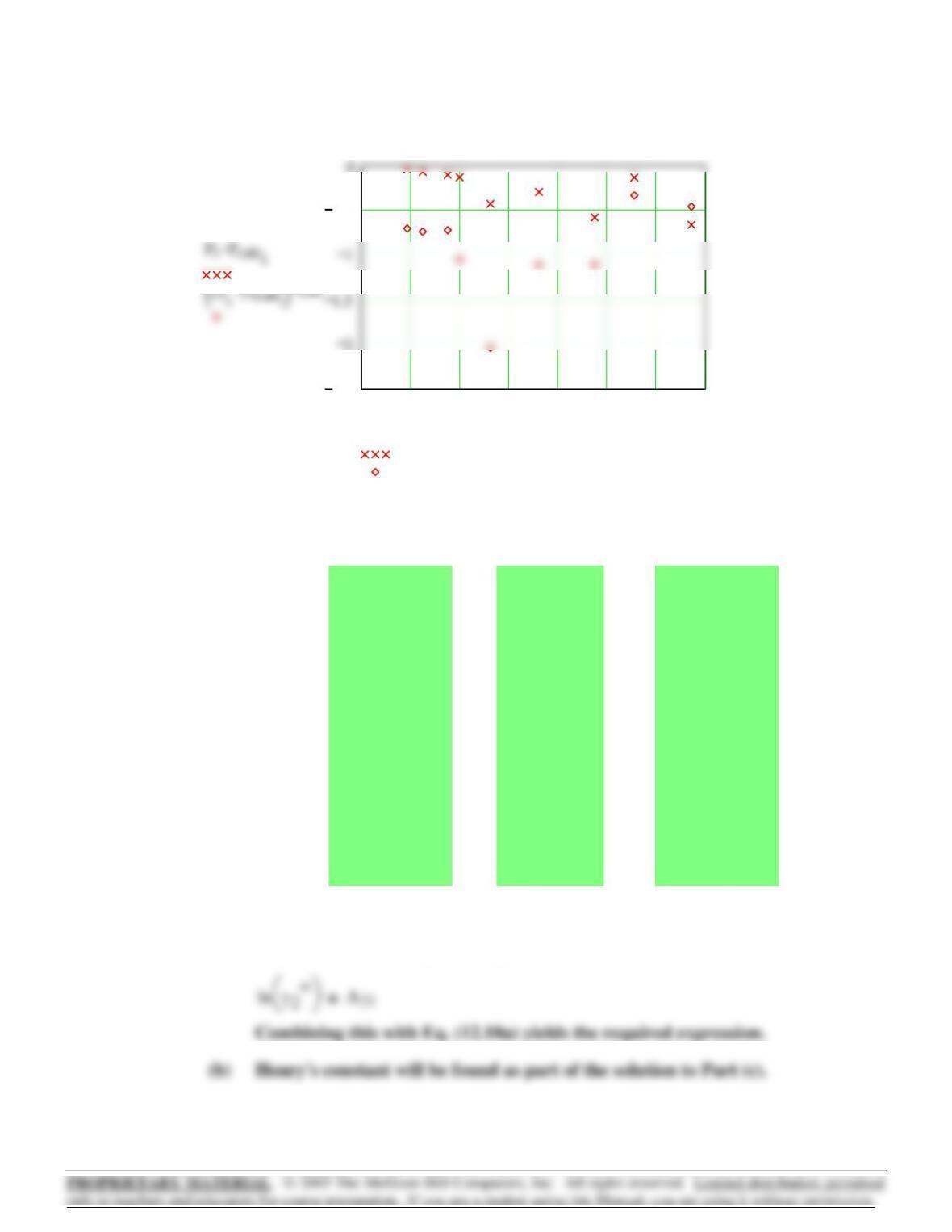
0 0.1 0.2 0.3 0.4 0.5 0.6 0.7
2.5
0.5
Pressure residuals
y1 residuals
x1i
553
0
iA12
Pix1iγ1x1ix2i
,A12
,A21
,
()
⋅Psat1
⋅
x2iγ2x1ix2i
,A12
,A21
,
()
⋅H2
exp A21
()
⋅+
…
⎛
⎜
⎜
⎜
⎝
⎞
⎟
⎠
−
⎡
⎢
⎢
⎢
⎣
⎤
⎥
⎥
⎥
⎦
2
d
d
⎡
⎢
⎢
⎢
⎣
⎤
⎥
⎥
⎥
⎦
∑
=
Given
The most satisfactory procedure for reduction of this set of data is to
find the value of Henry’s constant by regression along with the
Margules parameters.
BARKER’S METHOD by non-linear least squares.
Margules equation.
(c)
554
⎜
⎜
⎜
⎜
⎜
⎢
⎢
⎥
⎥
⎢
⎢
⎥
⎥
⎜
⎜
⎢
⎢
⎥
⎥
⎢
⎢
⎥
⎥
(d) γ1x1x2,( ) exp x22A12 2A
21 A12
−
()
⋅x1⋅+
⎡
⎣
⎤
⎦
⋅
⎡
⎣
⎤
⎦
:=
γ2x1x2,( ) exp x12A21 2A
12 A21
−
()
⋅x2⋅+
⎡
⎣
⎤
⎦
⋅
⎡
⎣
⎤
⎦
:=
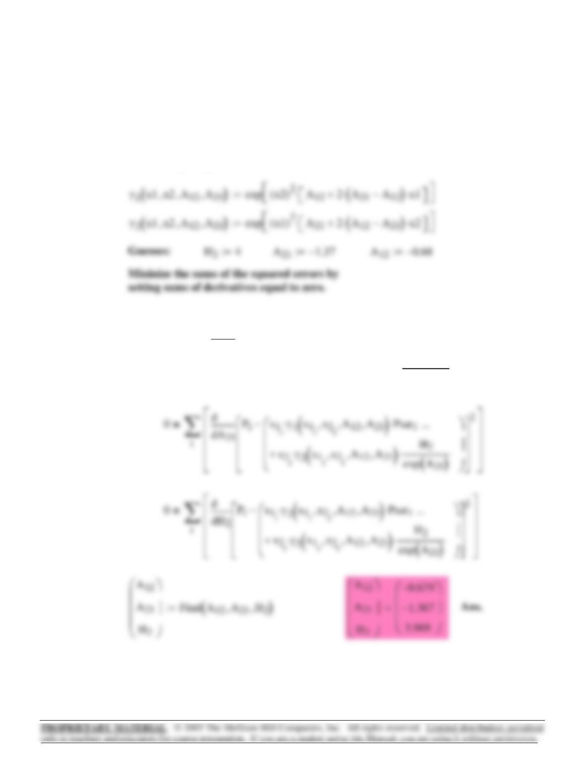
0 0.2 0.4 0.6 0.8
2
1
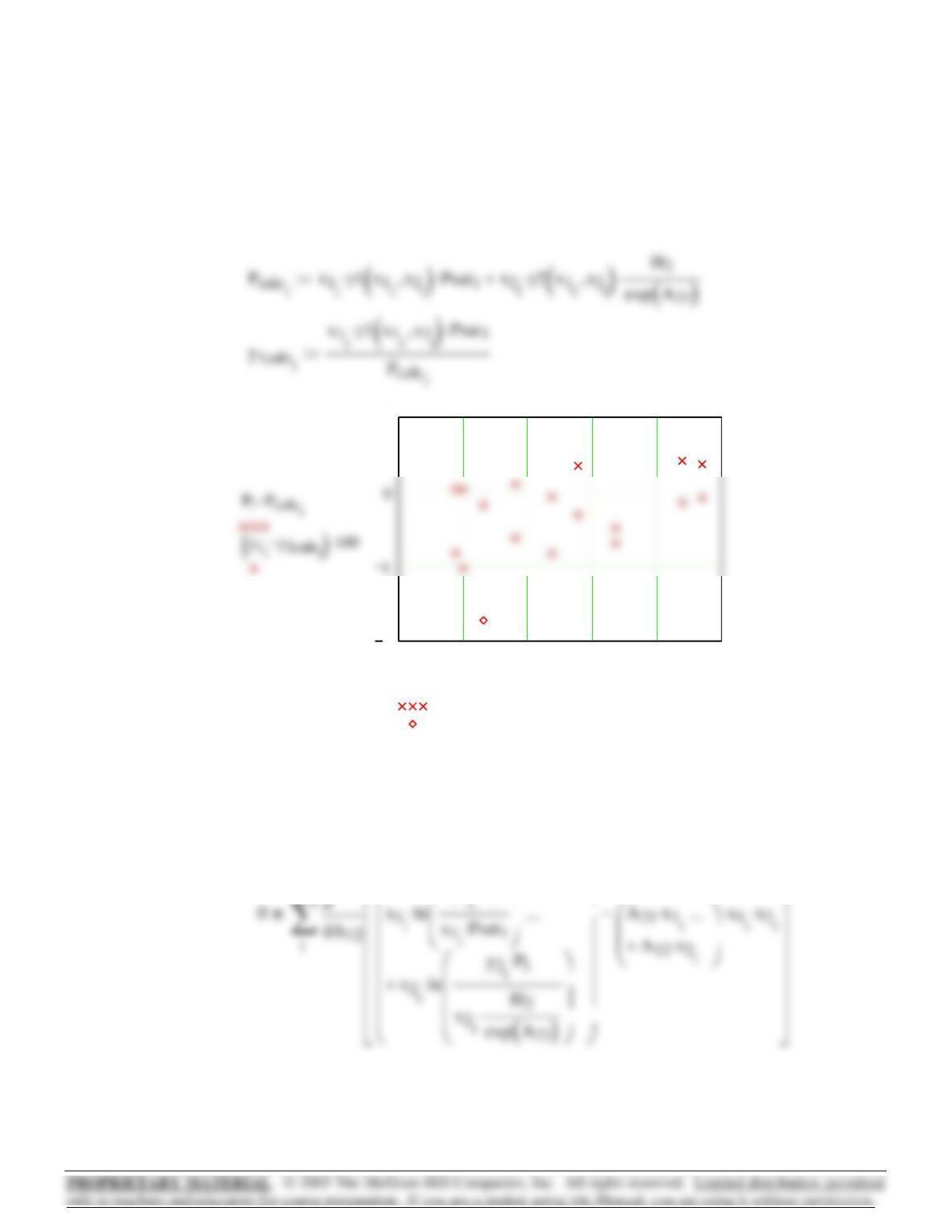
Pressure residuals
y1 residuals
x1i
Fit GE/RT data to Margules eqn. by least squares:
i19..:= y21y
1
−:=
Given
⎜
y1iPi
⋅
⎛
⎞
⎛
⎞
⎡
⎤
2
555
0
x1iln
y1iPi
⋅
x1iPsat1
⋅
⎛
⎜
⎜
⎞
⋅
…
⎛
⎜
⎜
⎞
⎟
A21 x1i
⋅
…
⎛
⎜
⎞
x1i
⋅x2i
⋅−
⎡
⎢
⎢
⎤
⎥
⎥
2
d
d
∑
=
0
iH2
x1iln
y1iPi
⋅
x1iPsat1
⋅
⎛
⎜
⎜
⎝
⎞
⎠
⋅
⎜
⎜
⎜
⎜
⎜
y2iPi
⋅
⎛
⎜
⎞
…
⎛
⎜
⎜
⎜
⎜
⎞
⎟
⎟
⎟
A21 x1i
⋅
A12 x2i
⋅+
…
⎛
⎜
⎜
⎝
⎞
⎠
x1i
⋅x2i
⋅−
⎡
⎢
⎢
⎢
⎢
⎤
⎥
⎥
⎥
⎥
2
d
d
∑
=
γ1x1x2,( ) exp x22A12 2A
21 A12
−
()
⋅x1⋅+
⎡
⎣
⎤
⎦
⋅
⎡
⎣
⎤
⎦
:=
⎡
⎣
⎤
⎦
⎡
⎣
⎤
⎦
556
⎜
⎜
⎜
Data reduction with the Margules equation and Eq. (10.5):
y2i1y
1i
−:=x2i1x
1i
−:=i1n..:=n9=n rows P():=
γ2
1.009
1.026
1.050
1.078
1.105
1.135
1.163
1.189
1.268
⎛
⎜
⎜
⎜
⎜
⎜
⎜
⎜
⎜
⎜
⎜
⎜
⎝
⎞
⎟
⎟
⎟
⎟
⎟
⎟
⎟
⎟
⎟
⎠
:=
γ1
1.304
1.188
1.114
1.071
1.044
1.023
1.010
1.003
0.997
⎛
⎜
⎜
⎜
⎜
⎜
⎜
⎜
⎜
⎜
⎜
⎜
⎝
⎞
⎟
⎟
⎟
⎟
⎟
⎟
⎟
⎟
⎟
⎠
:=
y1
0.2716
0.4565
0.5934
0.6815
0.7440
0.8050
0.8639
0.9048
0.9590
⎛
⎜
⎜
⎜
⎜
⎜
⎜
⎜
⎜
⎜
⎜
⎜
⎝
⎞
⎟
⎟
⎟
⎟
⎟
⎟
⎟
⎟
⎟
⎠
:=
x1
0.0895
0.1981
0.3193
0.4232
0.5119
0.6096
0.7135
0.7934
0.9102
⎛
⎜
⎜
⎜
⎜
⎜
⎜
⎜
⎜
⎜
⎜
⎜
⎝
⎞
⎟
⎟
⎟
⎟
⎟
⎟
⎟
⎟
⎟
⎠
:=
P
15.51
18.61
21.63
24.01
25.92
27.96
30.12
31.75
34.15
⎛
⎜
⎜
⎜
⎜
⎜
⎜
⎜
⎜
⎜
⎜
⎜
⎝
⎞
⎟
⎟
⎟
⎟
⎟
⎟
⎟
⎟
⎟
⎠
kPa:=
Data from Table 12.1(a)14.8
0 0.2 0.4 0.6 0.8
2
1
Pressure residuals
y1 residuals
x1i
557
B12 1150−cm3
mol
:=B22 1800−cm3
mol
:=B11 1840−cm3
mol
:=
Data reduction with the Margules equation and Eq. (14.1):
0.1
x1ix1,
A21 0.3:=A12 0.1:=
Guess:
GERTix1iln γ1i
()
⋅x2iln γ2i
()
⋅+:=i1n..:=
558