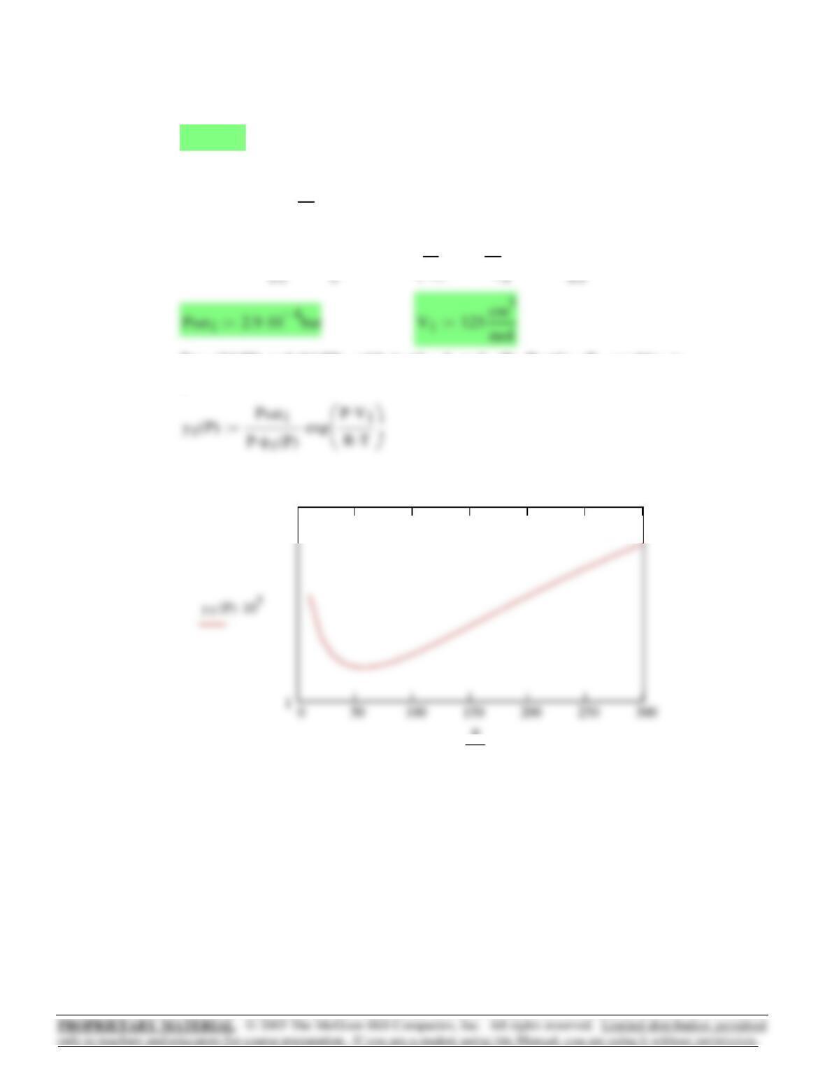
Find the conditions for VLLE:
Guess: Pstar P1sat:= y1star 0.5:=
Given Pstar x1βγ1x1β
()
⋅P1sat⋅1x1α−
()
γ2x1α
()
⋅P2sat⋅+=
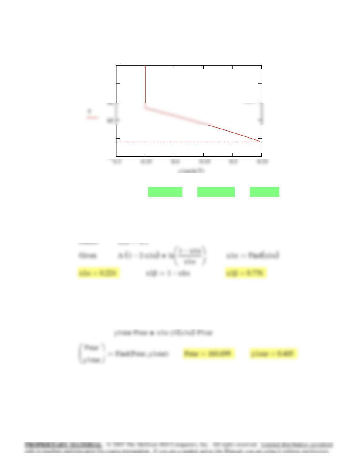
Calculate VLE in two-phase region.
Modified Raoult’s law; vapor an ideal gas.
Guess: x1 0.1:= P50:=
80
95
100
Tstar
Tdew
14.26 Pressures in kPa. P1sat 75:= P2sat 110:= A 2.25:=
γ1x1( ) exp A 1 x1−()
2
⋅
⎡
⎣
⎤
⎦
:= γ2x1( ) exp A x12
⋅
()
:=
Find the solubility limits:
577
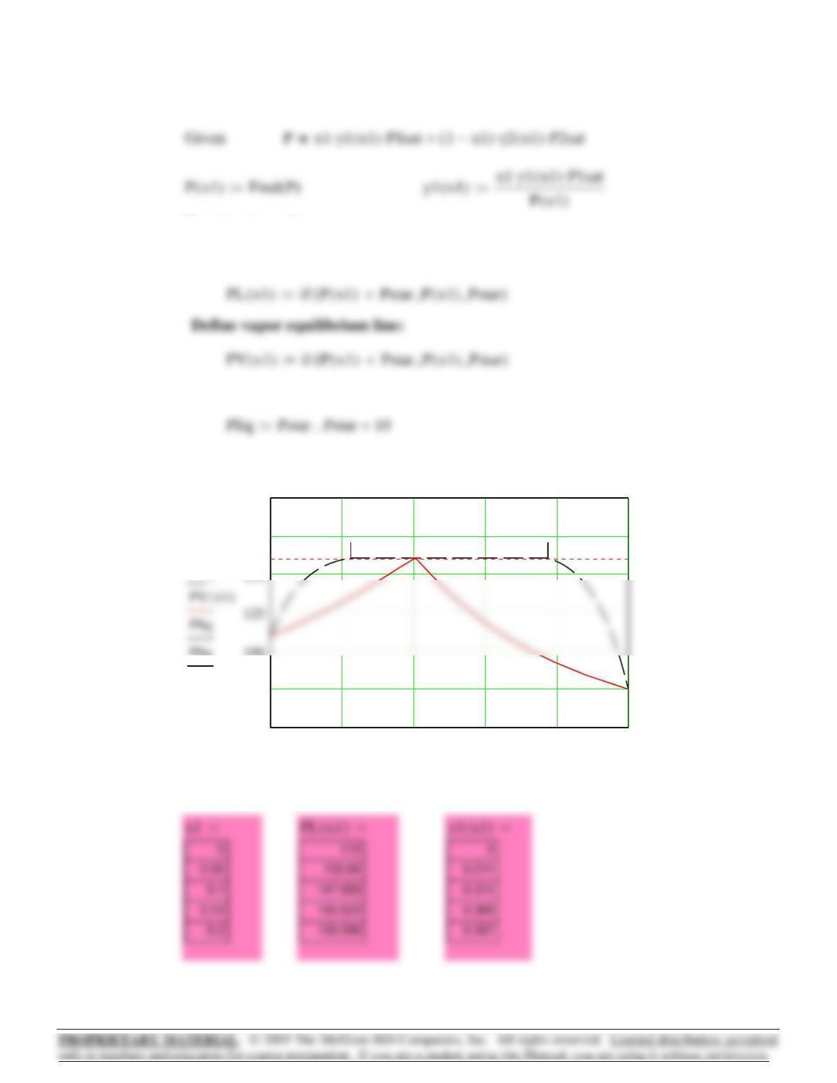
x1 0 0.05,0.2..:=
0 0.2 0.4 0.6 0.8 1
50
75
100
175
200
Pstar
PL x1()
Pliq
x1 y1 x1(),x1α, x1β,
x1 0 0.01,1..:=
Define pressures for liquid phases above Pstar:
Define liquid equilibrium line:
Plot the phase diagram.
578

z2 0.30:= z3 1 z1−z2−:=
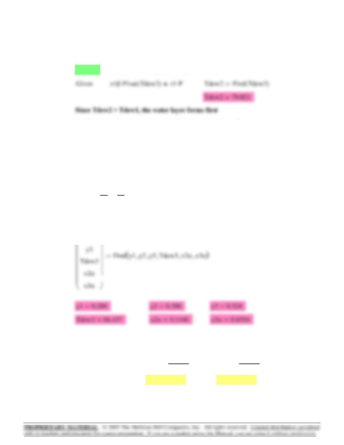
(a) Calculate dew point T and liquid composition
assuming the hydrocarbon layer forms first:
Guess: Tdew1 100:= x2αz2:= x3α1x2α−:=
Given Px2αP2sat Tdew1()⋅x3αP3sat Tdew1()⋅+=
z3 P⋅x3αP3sat Tdew1()⋅=
14.27 Temperatures in deg. C; pressures in kPa.
Water: P1sat T( ) exp 16.3872 3885.70
T 230.170+
−
⎛
⎜
⎝
⎞
⎠
:=
n-Pentane: P2sat T( ) exp 13.7667 2451.88
T 232.014+
−
⎛
⎜
⎝
⎞
⎠
:=
n-Heptane: P3sat T( ) exp 13.8622 2910.26
T 216.432+
−
⎛
⎜
⎝
⎞
⎠
:=
P 101.33:= z1 0.45:=
579
y1 P⋅P1sat Tdew3()=
y2
y3
z2
z3
=y1 y2+y3+1=
y2 P⋅x2αP2sat Tdew3()⋅=x2αx3α+ 1=
y1
y2
⎛
⎜
⎜
⎞
⎟
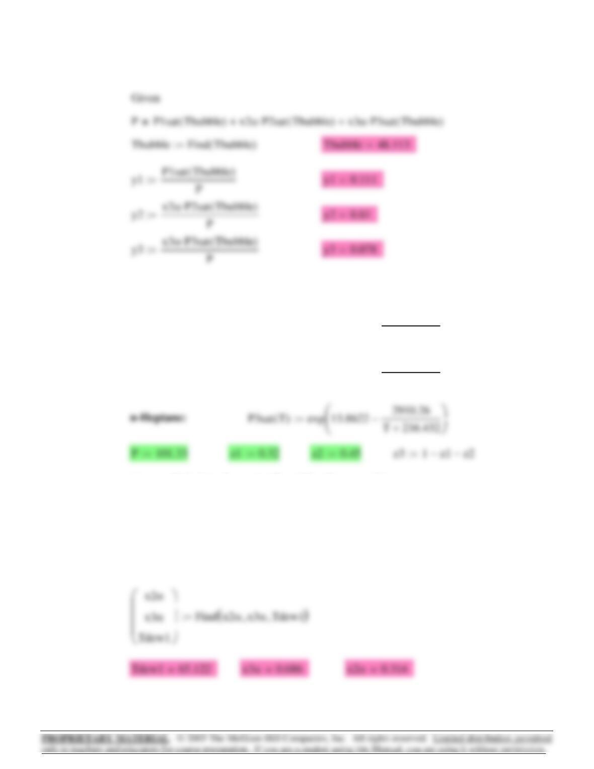
(c) Calculate the bubble point given the total molar composition of the
two phases
Tbubble Tdew3:= x2αz2
z2 z3+
:= x3αz3
z2 z3+
:=
x2α0.545=x3α0.455=
Calculate dew point temperature assuming the water layer forms first:
x1β1:= Guess: Tdew2 100:=
(b) Calculate the temperature at which the second layer forms:
Guess: Tdew3 100:= x2αz2:= x3α1x2α−:=
y1 z1:= y2 z2:= y3 z3:=
Given P P1sat Tdew3()x2αP2sat Tdew3()⋅+ x3αP3sat Tdew3()⋅+=
580
(a) Calculate dew point T and liquid composition
assuming the hydrocarbon layer forms first:
Guess: Tdew1 70:= x2αz2:= x3α1x2α−:=
Given Px2αP2sat Tdew1()⋅x3αP3sat Tdew1()⋅+=
z3 P⋅x3αP3sat Tdew1()⋅=x2αx3α+ 1=
14.28 Temperatures in deg. C; pressures in kPa.
Water: P1sat T( ) exp 16.3872 3885.70
T 230.170+
−
⎛
⎜
⎝
⎞
⎠
:=
n-Pentane: P2sat T( ) exp 13.7667 2451.88
T 232.014+
−
⎛
⎜
⎝
⎞
⎠
:=
581
⎜
y1 P⋅P1sat Tdew3()=y2
y3
z2
z3
=y1 y2+y3+1=
y2 P⋅x2αP2sat Tdew3()⋅=x2αx3α+ 1=
y1
y2
⎛
⎜
⎜
⎞
⎟
(c) Calculate the bubble point given the total
molar composition of the two phases
Tbubble Tdew3:= x2αz2
z2 z3+
:= x3αz3
z2 z3+
:=
x2α0.662=x3α0.338=
Calculate dew point temperature assuming the water layer forms first:
x1β1:= Guess: Tdew2 70:=
(b) Calculate the temperature at which the second layer forms:
Guess: Tdew3 100:= x2αz2:= x3α1x2α−:=
y1 z1:= y2 z2:= y3 z3:=
Given P P1sat Tdew3()x2αP2sat Tdew3()⋅+ x3αP3sat Tdew3()⋅+=
582
From Table 3.1, p. 98 of text:
σ1:= ε 0:= Ω 0.08664:= Ψ 0.42748:=
α1 0.480 1.574 ω⋅+ 0.176 ω2
⋅−
()
1Tr
0.5
−
()
⋅+
⎡
⎣
⎤
⎦
2
→
⎯
⎯⎯⎯⎯⎯⎯⎯⎯⎯⎯⎯⎯⎯⎯⎯⎯⎯⎯
⎯
:=
Given P P1sat Tbubble()x2αP2sat Tbubble()⋅+ x3αP3sat Tbubble()⋅+=
14.32 ω0.302
0.224
⎛
⎜
⎝
⎞
⎠
:= Tc 748.4
304.2
⎛
⎜
⎝
⎞
⎠K:= Pc 40.51
73.83
⎛
⎜
⎝
⎞
⎠bar:=
P 10bar 20bar,300bar..:=
T 353.15K:= Tr T
Tc
→
⎯
:=
Use SRK EOS
583
⎯
⎯
⎯
⎯
⎜
0 50 100 150 200 250 300
1.10 4
0.01
0.1
P
bar
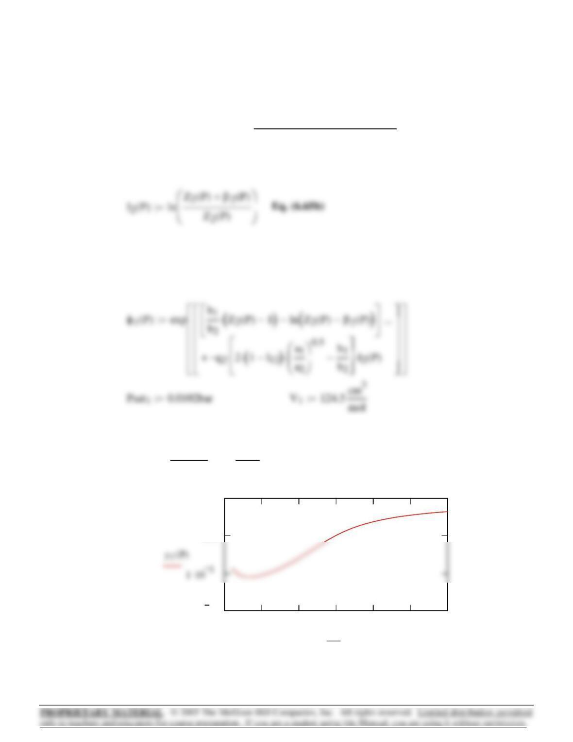
y1P() Psat1
Pφ1P()⋅exp PV
1
⋅
RT⋅
⎛
⎜
⎝
⎞
⎠
⋅:=
Eqs. (14.98) and (14.99), with φsat1 = 1 and (P – Psat1) = P, combine to give:
l12 0.088:=
Eq. (14.103):
For simplicity, let φ1 represent the infinite-dilution value of the fugacity
coefficient of species 1 in solution.
Z2P( ) Find z2
()
:=
Eq. (14.36)
z21β2P()+q2β2P()⋅z2β2P()−
z2εβ
2P()⋅+
()
z2σβ
2P()⋅+
()
⋅
⋅−=
Given
584
a7.298
0.067
⎛
⎜
⎝
⎞
⎠
kg m5
s2mol2
=b1.331 10 4−
×
2.674 10 5−
×
⎛
⎜
⎜
⎝
⎞
⎠
m3
mol
=
β2P() b2P⋅
RT⋅
:= Eq. (14.33) q2
a2
b2R⋅T⋅
:= Eq. (14.34)
z21:= (guess)
Given
14.33 ω0.302
0.038
⎛
⎜
⎝
⎞
⎠
:= Tc 748.4
126.2
⎛
⎜
⎝
⎞
⎠K:= Pc 40.51
34.00
⎛
⎜
⎝
⎞
⎠bar:=
P 10bar 20bar,300bar..:=
T 308.15K:= (K) Tr T
Tc
→
⎯
:=
Use SRK EOS
From Table 3.1, p. 98 of text:
σ1:= ε 0:= Ω 0.08664:= Ψ 0.42748:=
α1 0.480 1.574 ω⋅+ 0.176 ω2
⋅−
()
1Tr
0.5
−
()
⋅+
⎡
⎣
⎤
⎦
2
→
⎯
⎯⎯⎯⎯⎯⎯⎯⎯⎯⎯⎯⎯⎯⎯⎯⎯⎯⎯
⎯
:=
585
⎯
⎯
⎯
⎯
l12 0.0:= Eq. (14.103):
φ1P( ) exp b1
b2
Z2P() 1−
()
⋅ln Z2P() β2P()−
()
−
⎡
⎢
⎣
⎤
⎥
⎦
q2
−21 l
12
−
()
⋅a1
a2
⎛
⎜
⎝
⎞
⎠
0.5
⋅b1
b2
−
⎡
⎢
⎣
⎤
⎥
⎦
⋅I2P()⋅+
…
⎡
⎢
⎢
⎢
⎢
⎣
⎤
⎥
⎥
⎥
⎥
⎦
⎡
⎢
⎢
⎢
⎢
⎣
⎤
⎥
⎥
⎥
⎥
⎦
:=
Eqs. (14.98) and (14.99), with φsat1 = 1 and (P – Psat1) = P, combine to
give:
10
P
bar
Note: y axis is log scale.
586
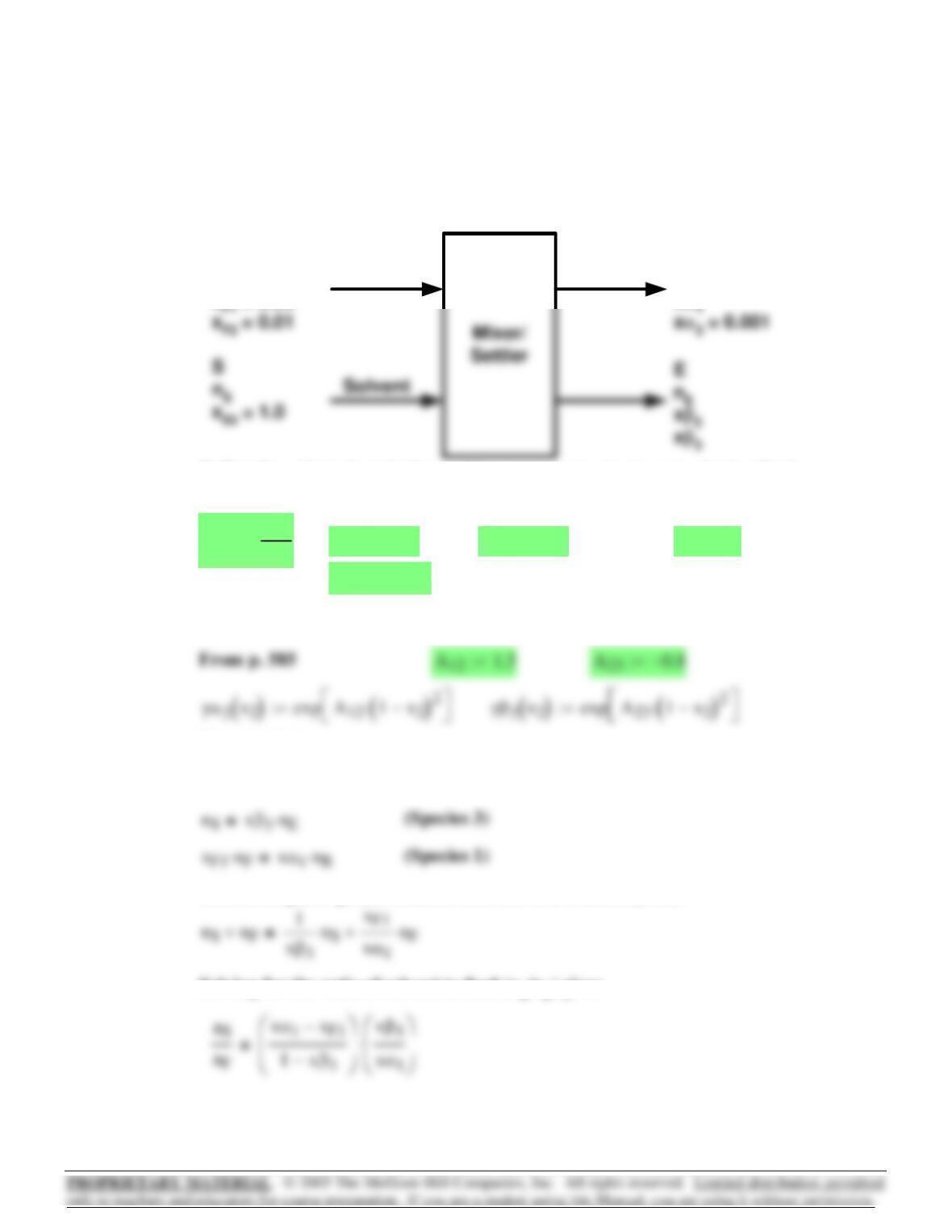
Solving for the ratio of solvent to feed (nS/nF) gives
Substituting the species balances into the total balance yields
(Total)
nSnF
+nEnR
+=
Material Balances
Appl
y
mole balances around the process as well as an equilibrium relationshi
p
xα11xα2
−:=xα20.001:=
xS3 1:=xF2 0.01:=xF1 0.99:=nF1mol
s
:=
Define the values given in the problem statement. Assume as a basis a feed
rate nF = 1 mol/s.
F
nF
xF1 = 0.99
R
nR
xα1
Feed
A labeled diagram of the process is given below. The feed stream is taken as
the α phase and the solvent stream is taken as the β phase.
14.45
587
xβ11xβ2
−:=xβ2
2
106
:=xα21xα1
−:=xα1
520
106
:=
Since this is a dilute system in both phases, Eqns. (C) and (D) from Example
14.4 on p. 584 can be used to find γ1
α and γ2
β.
1 – n-hexane
2 – water
14.46
nSnF
xα1xF1
−
1xβ3
−
⎛
⎜
⎝
⎞
⎠
xβ3
xα1
⎛
⎜
⎝
⎞
⎠
⋅:=
From above, the equation for the ratio nS/nF is:
⎣
⎦
⎣
⎦
Given
xβ20.5:=
Guess:
Solve for xβ2 using Mathcad Solve Block
⎣
⎦
⎣
⎦
Substituting for γα2 and γβ2
xα2γα2
⋅xβ2γβ2
⋅=
We need xβ3. Assume exiting streams are at equilibrium. Here, the only
distributing species is 2. Then
588
i12..:= j12..:= k12..:= x21x
1
−:= y21y
1
−:=
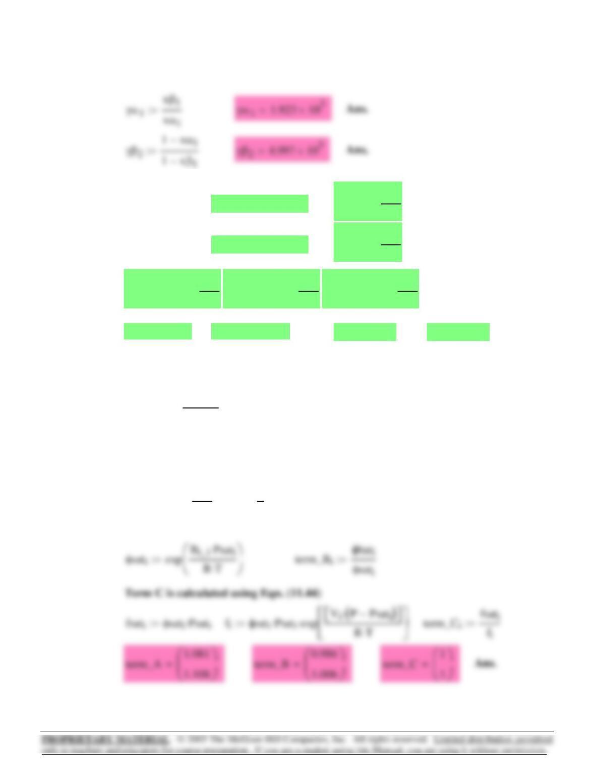
Term A is calculated using the given data.
term_Ai
yiP⋅
xiPsati
⋅
:=
Term B is calculated using Eqns. (14.4) and (14.5)
δji,2B
ji,
⋅Bjj,
−Bii,
−:=
φhatiexp P
RT⋅Bii,1
2
jk
yjyk
⋅2δji,δjk,
−
()
⋅
⎡
⎣
⎤
⎦
∑
⎡
⎢
⎣
⎤
⎥
⎦
∑
⎡
⎢
⎣
⎤
⎥
⎦
⋅+
⎡
⎢
⎢
⎣
⎤
⎥
⎥
⎦
⋅
⎡
⎢
⎢
⎣
⎤
⎥
⎥
⎦
:=
14.50 1 – butanenitrile Psat10.07287bar:= V190 cm3
mol
:=
2- benzene Psat20.29871bar:= V292 cm3
mol
:=
B11,7993−cm3
mol
:= B22,1247−cm3
mol
:= B12,2089−cm3
mol
:= B21,B12,
:=
T 318.15K:= P 0.20941bar:= x10.4819:= y10.1813:=
589
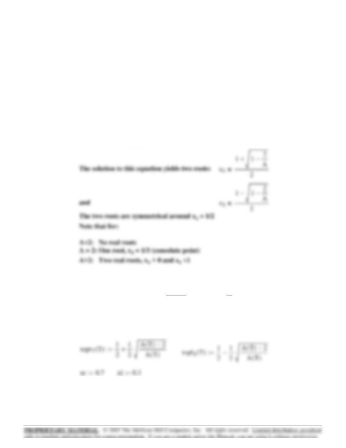
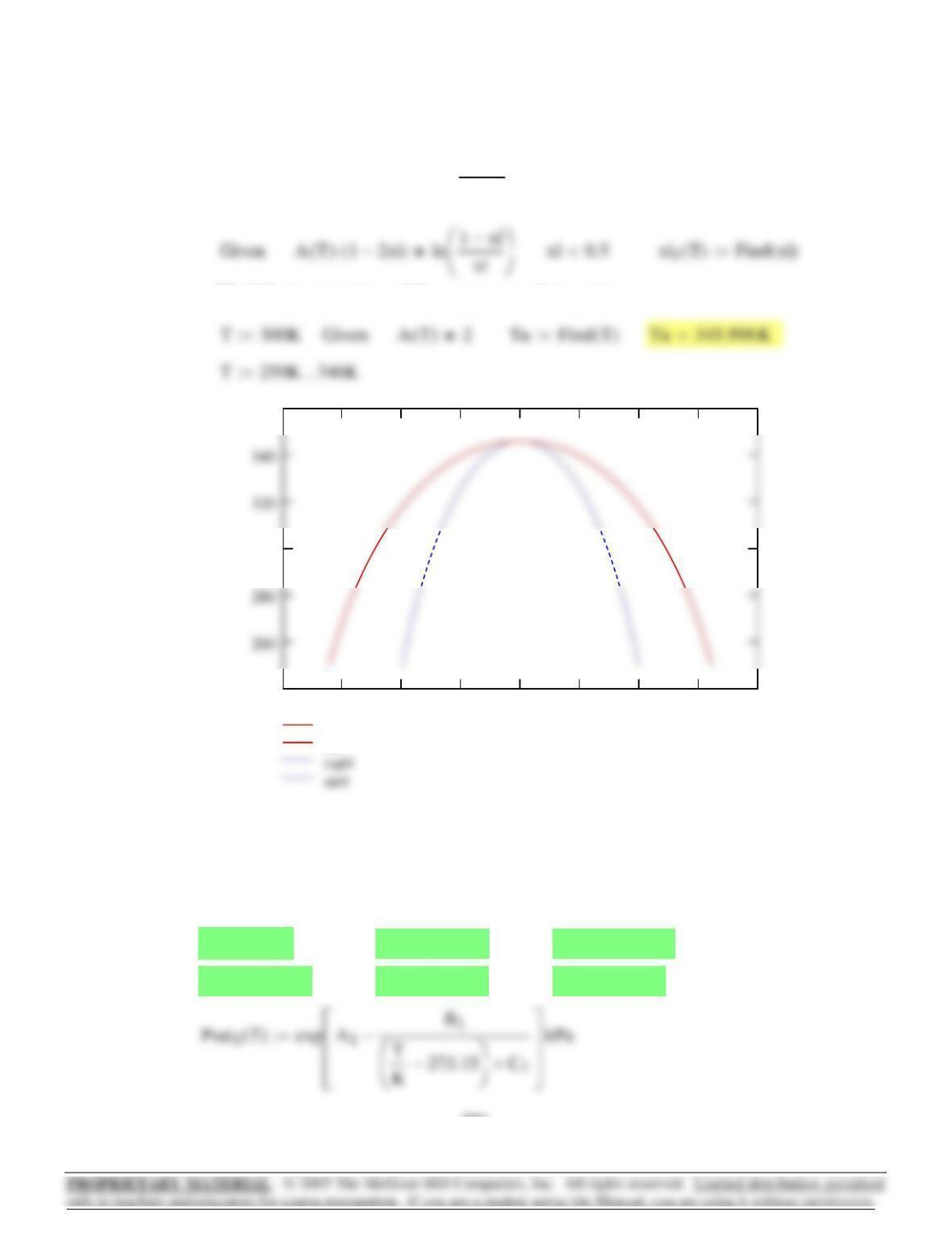
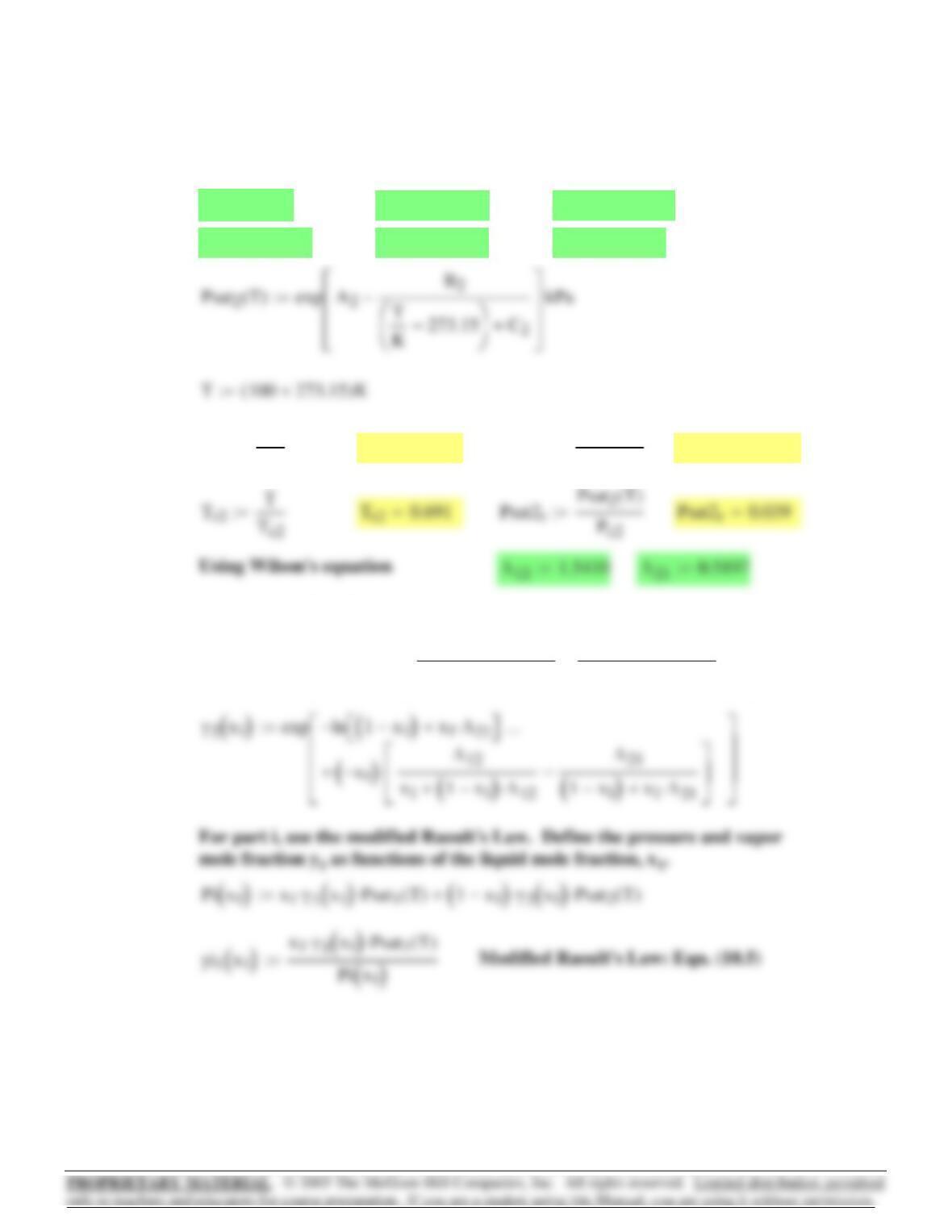
From Eq. (E) in Example 14.5, the solubility curves are solved using
a Solve Block:
From above, the equations for the spinodal curves are:
Both curves are symmetrical around x1 = 1/2. Create functions to
represent the left and right halves of the curves.
AT() 540−K
T21.1+3ln T
K
⎛
⎜
⎝
⎞
⎠
−:=
From Fig. 14.15:
Plot the spinodal curve along with the solubility curve b)
Substituting for x2: x1-x12 = 1/(2A) or x12-x1+1/(2A) = 0.
Thus, -2A = -1/x1x2 or 2Ax1x2 = 1.
For GE/RT = Ax1x2 = A(x1-x12)
d(GE/RT)/dx1 = A(1-2x1)
d2(GE/RT)/dx12 = -2A
Equivalent to d2(∆G/RT)/dx1
2 = 0, use d2(GE/RT)/dx1
2 = -1/x1x2
a)14.51
590
C1232.148:=B12914.23:=A114.0572:=
Pc1 45.60bar:=Tc1 556.4K:=ω10.193:=
1- Carbon tetrachloridef)
The solution is presented for one of the systems given. The solutions for the
other systems follow in the same manner.
14.54
0.1 0.2 0.3 0.4 0.5 0.6 0.7 0.8
240
300
360
xl1
xr1
Find the temperature of the upper consolute point.
⎜
xr1T( ) Find xr():=xr 0.5>AT( ) 1 2xr−()⋅ln 1xr−
xr
⎛
⎜
⎝
⎞
⎠
=Given
591
⎜
γ1x1
()
exp ln x11x
1
−
()
Λ12
⋅+
⎡
⎣
⎤
⎦
−
1x
1
−
()
Λ12
x11x
1
−
()
Λ12
⋅+
Λ21
1x
1
−
()
x1Λ21
⋅+
−
⎡
⎢
⎣
⎤
⎥
⎦
⋅+
…
⎡
⎢
⎢
⎢
⎣
⎤
⎥
⎥
⎥
⎦
:=
Psat1r0.043=Psat1r
Psat1T()
Pc1
:=Tr1 0.671=Tr1
T
Tc1
:=
⎢
⎥
C2216.432:=B22910.26:=A213.8622:=
Pc2 27.40bar:=Tc2 540.2K:=ω20.350:=
2 – n-heptane
592
⎡
⎣
⎤
⎦
⎢
⎥
⎢
⎢
⎥
⎥
yii1x1
()
fii x1
()
1
:=
Pii x1
()
fii x1
()
0
:=
fii is a vector containing the values of P and y1. Extract the pressure, P and
vapor mole fraction, y1 as functions of the liquid mole fraction.
y1φ1P()⋅P⋅x1γ1x1
()
⋅Psat1T()⋅=
Given
P 1bar:=y10.5:=
Guess:
Solve Eqn. (14.1) for y1 and P given x1.
φsat10.946=φsat1PHIB Tr1 Psat1r
,ω
1
,
()
:=
For part ii, assume the vapor phase is an ideal solution. Use Eqn. (11.68)
and the PHIB function to calculate φhat and φsat.
593
0 0.2 0.4 0.6 0.8
1
1.1
1.6
1.7
2
Pi x1
()
bar
Pi x1
()
x1yi1x1
()
,x1
,yii1x1
()
,
594