st
n
st
yn
st
xn
AMM
)sincos(
where st
xn
M and st
yn
M are given in the solution to Problem
mLMmLM
mLMmLM
st
y
st
x
y
x
2672.04982.0
5758.00490.0
22
11
(b)
The peak values, M
n , of the modal contributions M
n(t)
to response M
are determined next
7. Combine peak modal responses.
(a) SRSS rule
2
sin21.5cos72.9
(c)
(b) CQC rule
Using Eq. (13.7.4), the CQC estimate for the peak value
of M
can be calculated:
where
8. Determine maximum of M
over
22
)sin(coscossin)(2
1
d
BCA
M
Therefore, the maximum value of M occurs for
that
satisfies
Substituting A, B, and C from Eq. (c) into Eq. (e) gives
rad8288.0,rad7420.0)5000.11(tan
1
5000.112tan
1
for 0.7420 rad, 9.38 k in.
M
1
147
(b) CQC rule
Substituting A, B, and C from Eq. (d) into Eq. (e) gives
9. Comments.
Modes 1 and 2 are strongly correlated (
12 = 0.9089);
Problem 13.69
Solve Problem 13.67 for ground motion in the z-direction.
Solution:
L
z
x
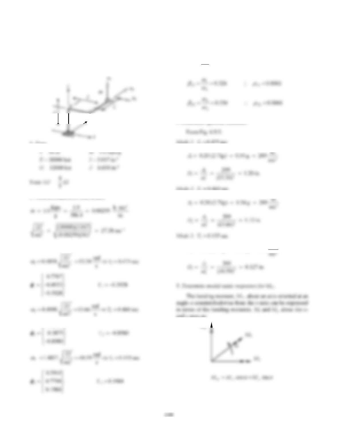
1. Data.
2. Natural frequencies and modes.
From Problems 10.28 and 13.29:
M
M
M
0.2084
3. Determine correlation coefficients.
Use Eq. (13.7.10) to compute ij
for
= 0.05:
9089.0969.0
12
2
1
12
Mode 1: 10.475 secT
Mode 2: 20.460 secT
32
in.
0.20 (2.71g) 0.54 g 209 sec
A
and y-axes as:
L
y
149
Therefore,
n
st
yn
st
xn
AMM
)sincos(
mLMmLM
mLMmLM
st
y
st
x
st
y
st
x
0785.01152.0
6192.01544.1
33
22
(b)
Equation (a) after substituting Eq. (b) becomes
2
sin08.12cos52.22
(c)
where
(b) CQC rule
8. Determine maximum of M
over
To find the value of
corresponding to the maximum
value of M, solve
(a) SRSS rule
ink98.25rad,5421.0for
M
150
(b) CQC rule
Substituting A, B, and C from Eq. (d) into Eq. (e) gives
9. Comments.
Modes 1 and 2 are strongly correlated (
12 = 0.9089);
151
y
x
1. Data.
L = 36 in. m = 1.0 kips/g
2. Natural frequencies and modes.
From Problems 10.28 and 13.30:
0.3928
M
M
3. Determine correlation coefficients.
Use Eq. (13.7.10) to compute ij
for
= 0.05:
0066.0336.0
23
3
2
23
1
209 1.20 in.
A
D
2
(13.66)
5. Determine modal static responses for M
.
m
z
a
uz
uy
152
Therefore,
MMM
sincos
where st
xn
M and st
yn
M are given in the solution to Problem
mLMmLM
st
y
st
x
2862.05335.0
22
(b)
The peak values, M
n, of the modal contributions M
n(t)
to response M are determined next
7. Combine peak modal responses.
82.38 k in. 260.20 k in. 214.25 k in.AB C
)coscossinsin(
CBA
where
8. Determine maximum of M
over
Therefore, the maximum value of M
occurs for
that
satisfies
Substituting A, B, and C from Eq. (c) into Eq. (e) gives
9732.12tan
153
(b) CQC rule
Substituting A, B, and C from Eq. (d) into Eq. (e) gives
9. Comments.
Modes 1 and 2 are strongly correlated (
12 = 0.9089);
Problem 13.71
Solution:
L
EI
2
u
1. Data.
62
12 ft, 50 kips/g, = 7.8 10 kip-inLm EI
0.849
m2m
Figure P13.71a
12
st n
b
Ps
For α = 30°
4. Response of modal SDF systems.
5. Response history analysis.
Substituting the modal static responses in Eq. (13.1.16)
gives the response history:
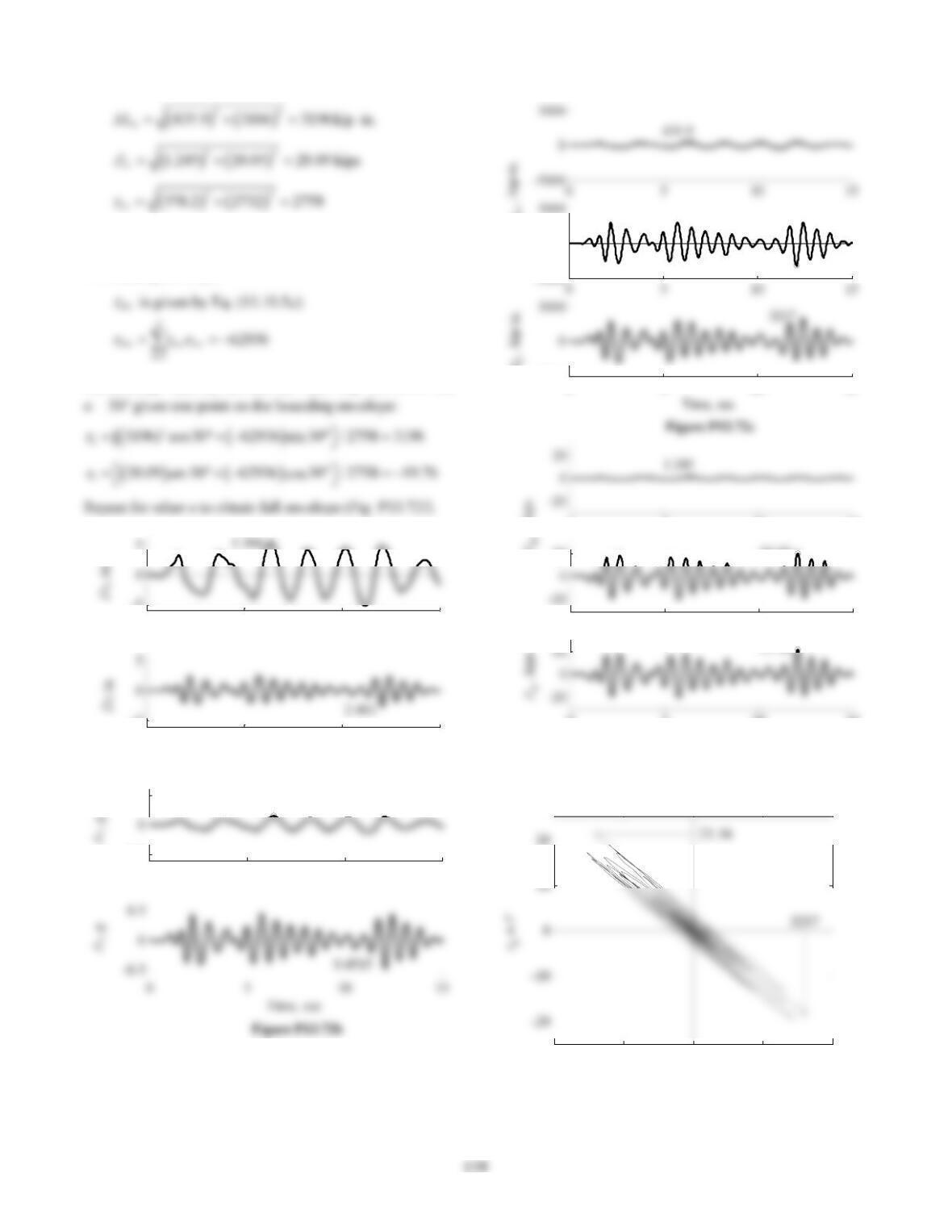
Results are plotted in Figs. P13.71c and P13.71d. Plotting
6. Response spectrum analysis.
Because the natural frequencies of this system are well
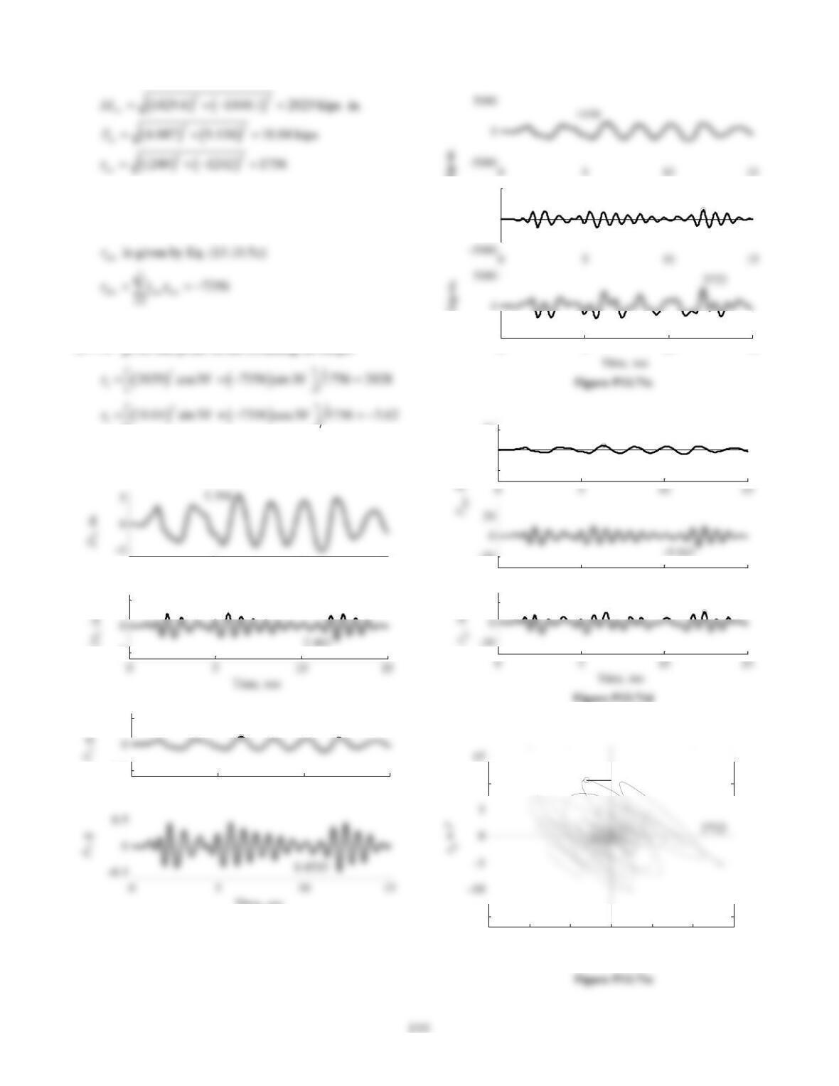
These estimates are shown in Fig. P13.71f.
7. Bounding envelope.
Substituting ,,,and
abo o bo o
rrr r
into Eq, (13.10.3) for
30
gives one point on the bounding envelope:
Repeat for other α to obtain full envelope in Fig. P13.71g.
Figure P13.71b
0 5 10 15
-5
5
0 5 10 15
-0.5
0.5 0.1376
Time, sec
0
5000
1440
M
bn
, kip-in.
0 5 10 15
-5000
M
b
, kip-in.
-20
0
20 4.087
0 5 10 15
-20
20
10.76
–3000 -2000 -1000 01000 2000 3000
-15
10
10.76
r
a
M
b
156
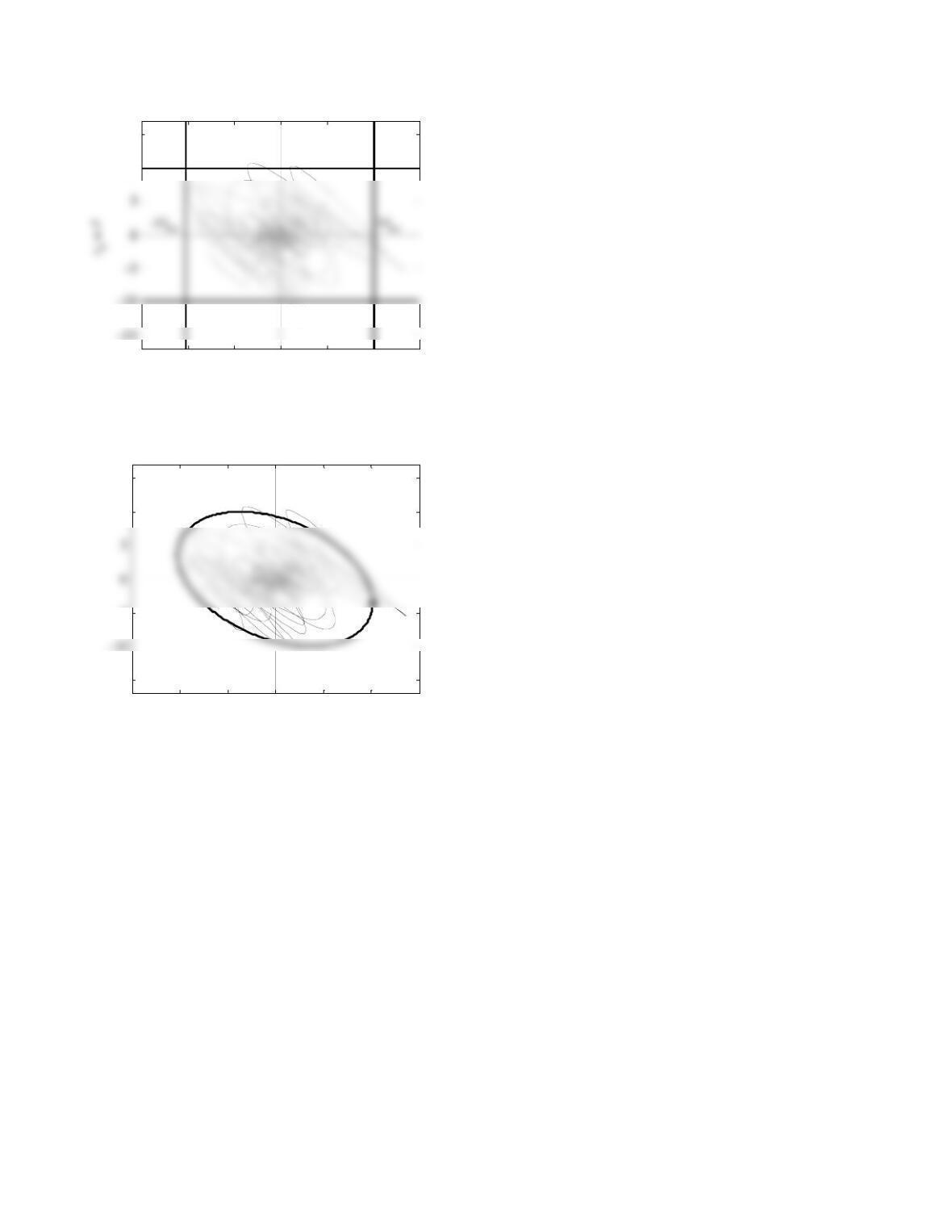
Figure P13.71f
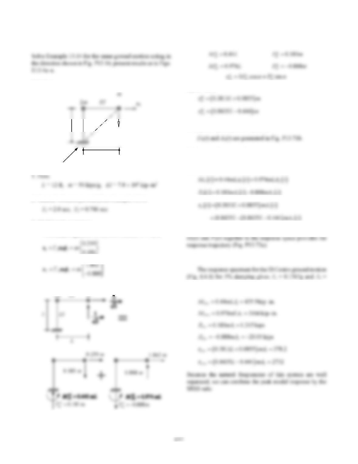
Figure P13.71g
–3000 -2000 -1000 01000 2000 3000
-10
10
15
r
a
M
b
P
o
-P
o
-3000 -2000 –1000 01000 2000 3000
-15
-5
10
15
(2028,-3.62)
r
a
M
b
Problem 13.72
Solution:
2. Natural vibration periods from Example 13.14.
3. Modal static responses.
The modal expansion of s (from Problem 13.16) is:
The modal static responses are as follows:
Figure P13.72a
st 12
nn
bn
M
sL sL
st 2
n
bn
Ps
For α = 30°,
4. Response of modal SDF systems.
5. Response history analysis.
Substituting these in Eq. (13.1.16) gives the response
history:
12
2
b
Results are plotted in Figs. P13.72c and P13.72d. Plotting
6. Response spectrum analysis.
0.4515g. Substituting for An, the modal static responses, m
and L gives the following peak modal values:
L
EI
u2
ug(t)
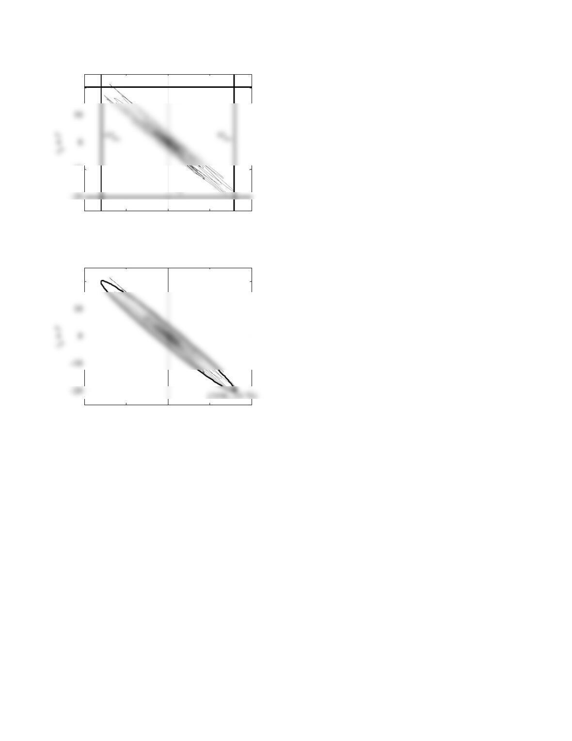
L
These estimates are shown in Fig. P13.72(f).
7. Bounding envelope.
Substituting ,,,and
abo ao bo o
rrr r
into Eq. (13.10.3) for
Figure P13.72d
Figure P13.72e
0 5 10 15
-5
0 5 10 15
-5
Time, sec
0 5 10 15
-0.5
0.5 0.1376
0
5000
-3166
M
bn , kip-in.
0 5 10 15
-5000
M
0 5 10 15
0 5 10 15
20 20.05
P
, kips
0 5 10 15
Time, sec
–4000 -2000 02000 4000
r
a
M
b
159
Figure P13.72f
Figure P13.72g
–4000 -2000 02000 4000
-10
20
r
a
M
b
P
o
-P
–4000 -2000 02000 4000
20
r
a
M
b