Chapter 13 Homework The CQC estimate of the peak response is close

109

CQC estimates of the peak displacements:

6. Determine peak bending moments.

Peak modal responses:

From the figure in the solution to Problem 13.15:

1

1.443 1.443 (0.00388) (120)

st

b

MmL



Hence,

SRSS estimate of the peak bending moment:

CQC estimate of the peak bending moment:

7. Comments.

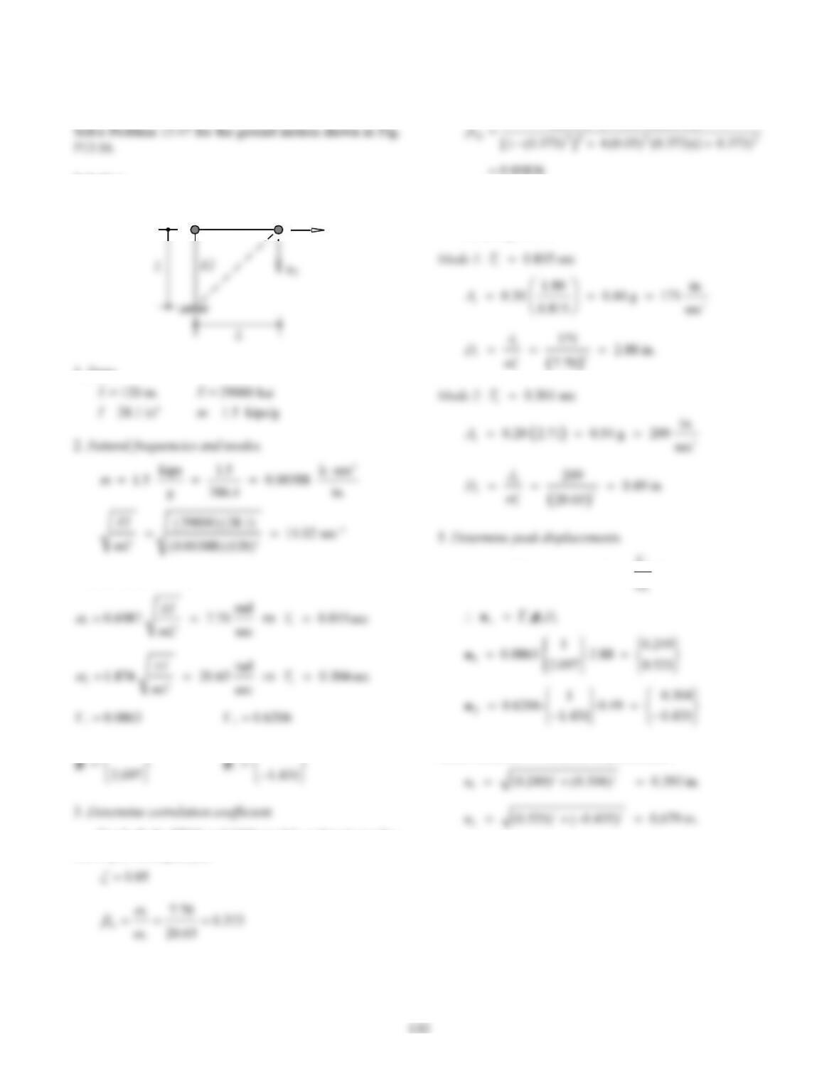
Problem 13.49

Solution:

1. Data.

From Problem 13.16:



1





Use both the SRSS and CQC modal combination rules.

For CQC, we require



12:

 From Eq. (13.7.10):

00836.0

)373.0()373.01()05.0(8

5.12





4. Determine spectral ordinates.

From Fig. 6.9.5:

2

un

st st

nnn n n

A





uu



SRSS estimates of the peak displacements:

2m m

EI

u1

111

CQC estimates of the peak displacements:

6. Determine peak bending moments.

Peak modal responses:

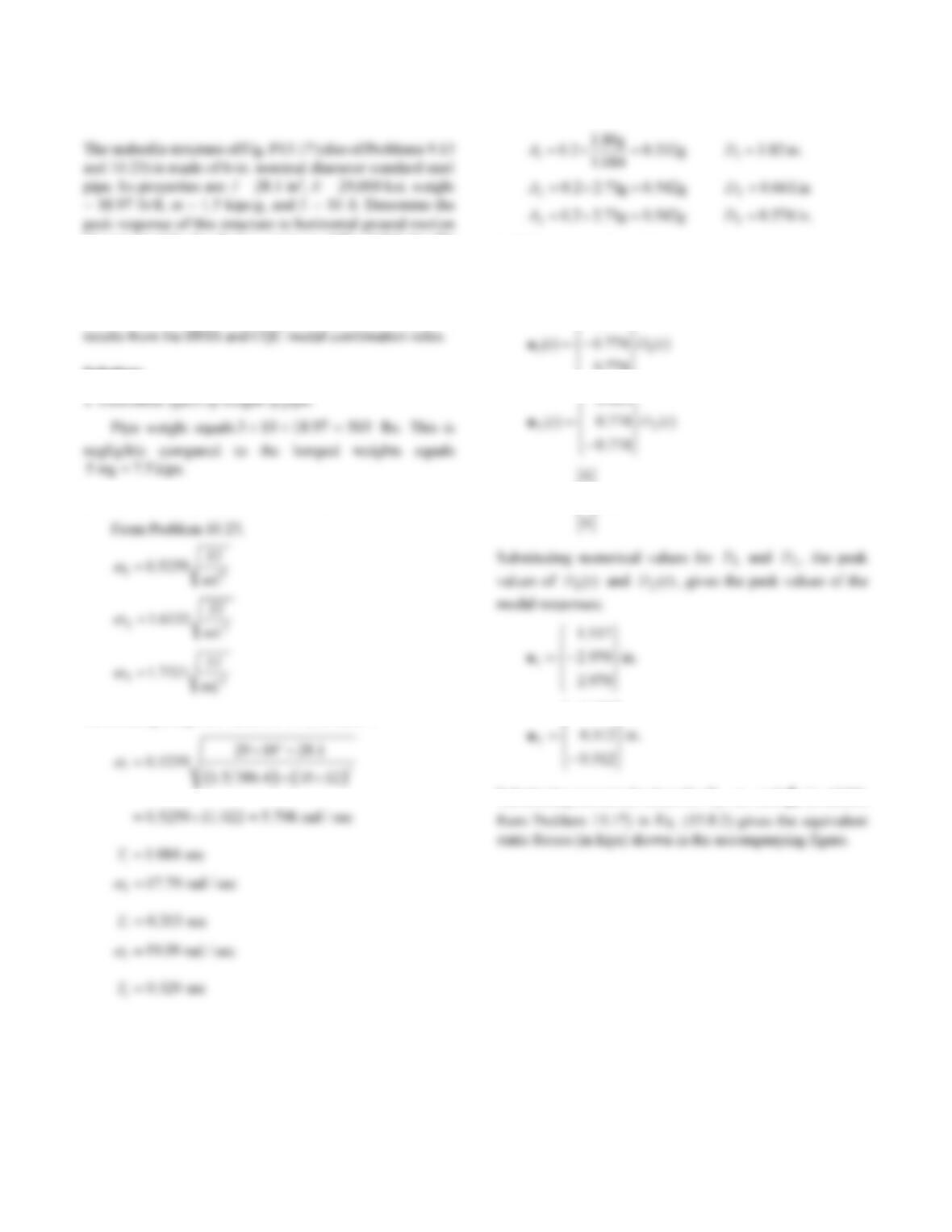
From the figure in the solution to Problem 13.16:

1

0.440 0.440 (0.00388) (120)

st

b

MmL



Hence,

SRSS estimate of the peak bending moment:

CQC estimate of the peak bending moment:

7. Comments.

112

Problem 13.50

characterized by the design spectrum of Fig. 6.9.5 (for 5%

damping) scaled to 0.20g peak ground acceleration.

Compute (a) displacements u1, u2, and u3, and (b) the

bending moments at the base of the column and at location

a of the beam. Comment on the differences between the

Solution:

2. Determine design spectrum ordinates.

Substituting the given values of , , , mIE and L:

For these n

T, the design spectrum of Fig. 6.9.5 gives

3. Determine peak modal responses.

The modal displacements, available from Problem

13.17, are

774.0

397.0









)(

0

)( 33 tDt 















u

399.0





Substituting numerical values for n

, m, and n



(available

113



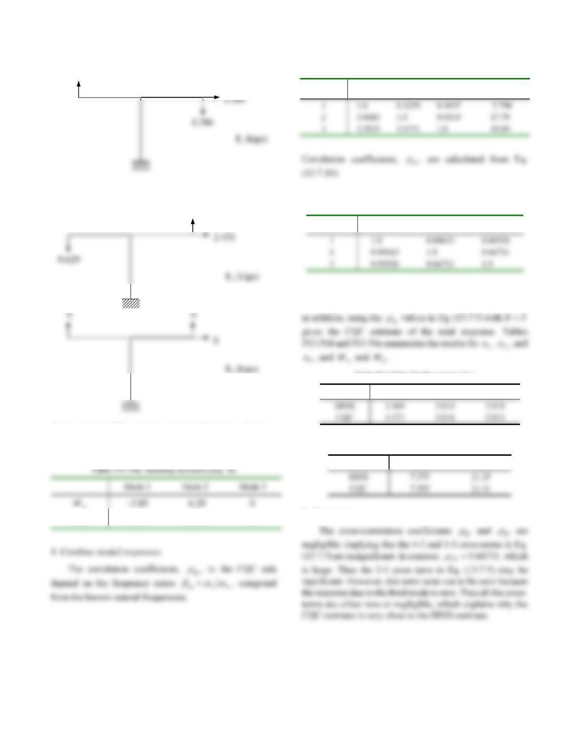
Static analysis of the structure subjected to forces n

f gives

the peak values of the bending moments (kip–ft) due to each

mode (Table P13.50a).

b

M 59.17 93.11 0

Table P13.50b: Natural frequency ratios, in



Mode, i 1



n 2n 3n (rad/sec)

i



Table P13.50c: Correlation coefficients, in



Mode, i 1



n 2n 3



n

Substituting the peak modal responses in Eq. (13.7.3) with

3



N gives the SRSS estimate of the total response, and,

Table P13.50d: Displacements (in.)

1

u 2

u 3

u

Table P13.50e: Bending moments (kip–ft)

a

M b

M

5. Comments.

386.0

629.0

3

114

Problem 13.51

Solve Problem 13.50 if the excitation is vertical ground

motion characterized by the design spectrum of Fig. 6.9.5

(for 5% damping) scaled to 0.20g peak ground acceleration.

Solution:

1. Determine design spectrum ordinates.

From the values obtained in Problem 13.50, we have

2. Determine peak modal responses.

(a) The modal displacements, available from Problem

13.18, are

Substituting numerical values for 3

D, the peak value of

)(

3tD , gives the peak values of the modal responses:

(b) Substituting numerical values for n

, m, and n



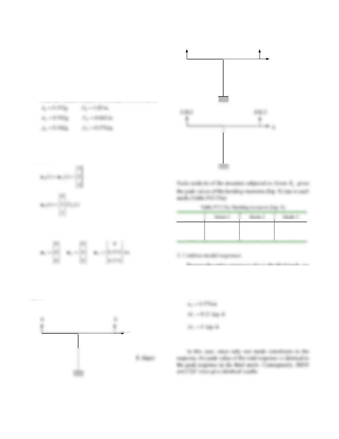
(available from Problem 13.18) in Eq. (13.8.2) gives the

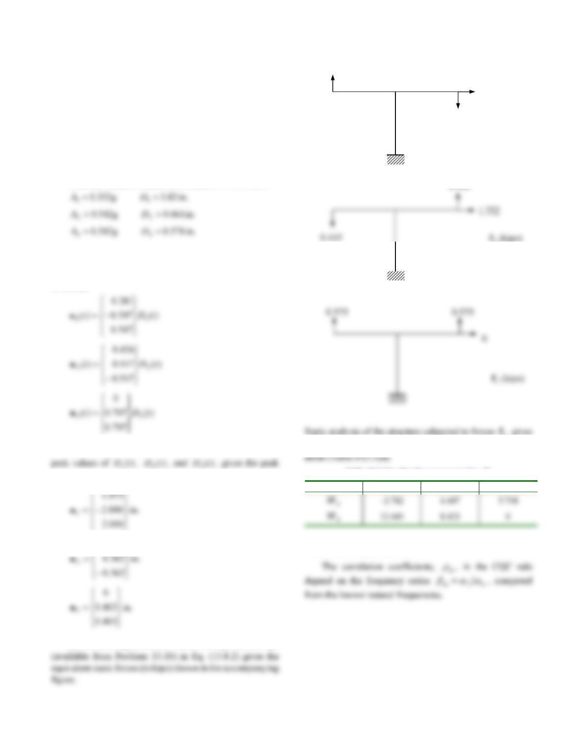
equivalent static forces (in kips) shown in the accompanying

figure.

a

M 0 0 8.13

M 0 0 0

Because the entire response is due to the third mode, we

do not need to combine modal responses. The total response

is the same as the third mode response:

in. 574.0

in. 0

2

1



u

4. Comments.

0

(kips)

2

f

(kips)

3

f

115

Problem 13.52

Solve Problem 13.50 if the excitation is ground motion in

the direction b–d, characterized by the design spectrum of

Fig. 6.9.5 (for 5% damping) scaled to 0.20g peak ground

acceleration.

Solution:

1. Determine design spectrum ordinates.

From the values obtained in Problem 13.50, we have

2. Determine peak modal responses.

(a) The modal displacements, available from Problem

13.19, are

Substituting numerical values for 1

D, 2

D, and 3

D, the

values of the modal responses:

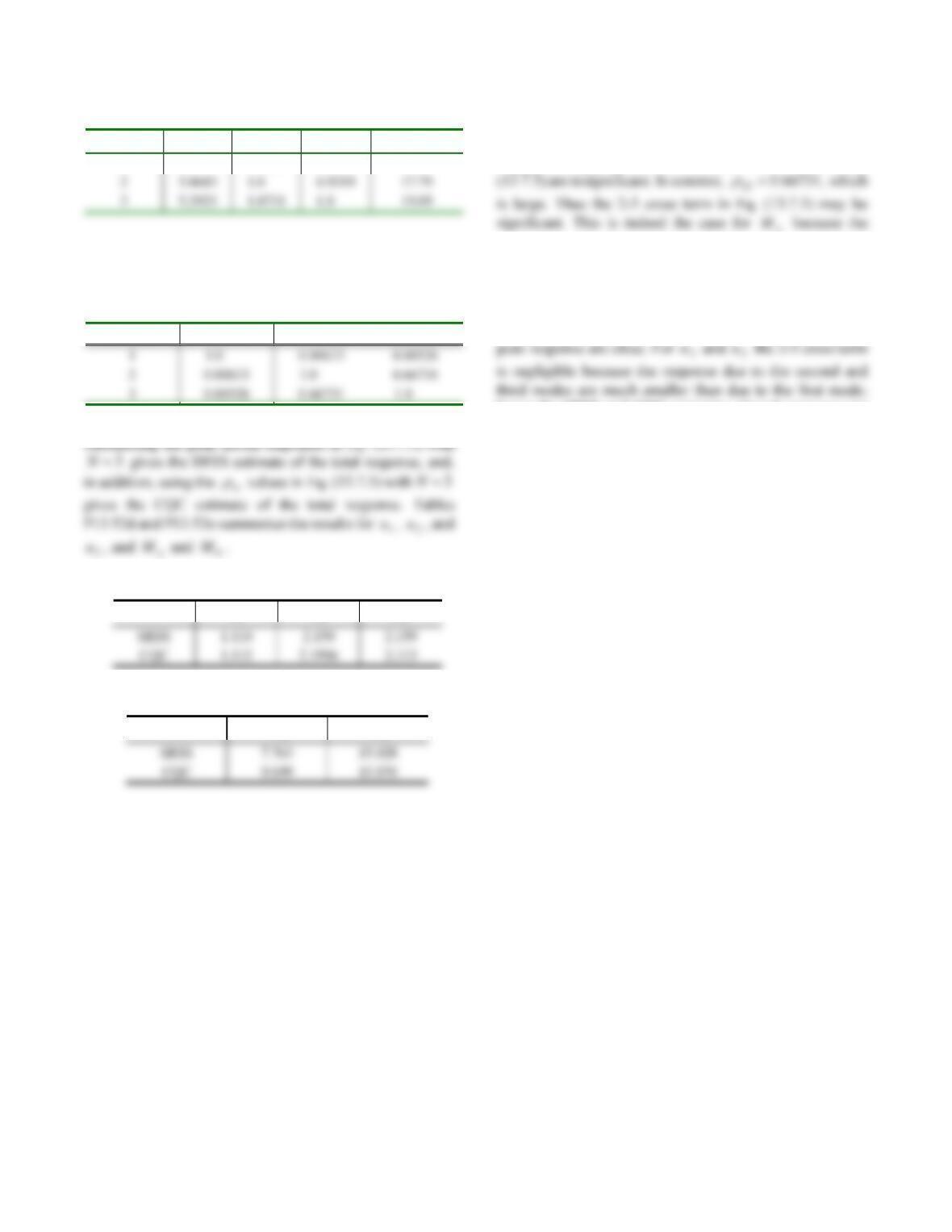
(b) Substituting numerical values for n

, m, and n



the peak values of the bending moments (kip–ft.) due to each

Table P13.52a: Bending moments (kip–ft)

Mode 1 Mode 2 Mode 3

3. Combine modal responses.

282.0









272.0

1.050

272.0

(kips)

1

f

2

116

Table P13.52b: Natural frequency ratios, in



Mode, i 1n 2n 3n (rad/sec)

i



1 1.0 0.3259 0.3037 5.798

Correlation coefficients, in



, are calculated from Eq.

(13.7.10):

Table P13.52c: Correlation coefficients, in



Mode, i 1n 2n 3



n



Table P13.52d: Displacements (in.)

1

u 2

u 3

u

Table P13.52e: Bending moments (kip–ft)

a

M b

M

4. Comments.

The cross-correlation coefficients 12



and 13



are

negligible, implying that the 1-2 and 1-3 cross-terms in Eq.

second and third mode contributions are significant.

Because the cross term is positive, the CQC estimate for

a

M is significantly larger than its SRSS estimate. For 1

u

and b

M the 2-3 cross term is zero because the third mode

response is zero; hence the SRSS and CQC estimates of

hence the SRSS and CQC estimates of peak response are

close.

Problem 13.53

Solve Problem 13.50 if the excitation is ground motion in

the direction b-c, characterized by the design spectrum of

Solution:

1. Determine design spectrum ordinates.

From the values obtained in Problem 13.50, we have

2. Determine peak modal responses.

426.0







Substituting numerical values for 1

D, 2

D, and 3

D, the

values of the modal responses:

073.1











282.0







0





(b) Substituting numerical values for n

, m, and n



Static analysis of the structure subjected to forces n

f gives

Table P13.53a: Bending moments (kip–ft)

Mode 1 Mode 2 Mode 3

b

The correlation coefficients, in



, in the CQC rule

depend on the frequency ratios niin





, computed

1.050

272.0

(kips)

f

Table P13.53b: Natural Frequency Ratios, in



Mode, i 1n 2n 3n (rad/sec)

i



Correlation coefficients, in



, are calculated from Eq.

(13.7.10):

Table P13.53c: Correlation coefficients, in



Mode, i 1n 2n 3



n

Substituting the peak modal responses in Eq. (13.7.3) with

3N gives the SRSS estimate of the total response, and,

in addition, using the in



values in Eq. (13.7.5) with 3



N

gives the CQC estimate of the total response. Tables

P13.53d and P13.53e summarize the results for 1

u, 2

u, and

3

u, and a

M and b

M.

Table P13.53d: Displacements (in.)

1

u 2

u 3

u

SRSS 1.110 2.159 2.159

Table P13.53e: Bending moments (kip–ft)

a

M b

M

4. Comments.

The cross-correlation coefficients 12



and 13



are

negligible, implying that the 1-2 and 1-3 cross-terms in Eq.

(13.7.5) are insignificant. In contrast, 66731.0

23 



, which

a

M is smaller than its SRSS estimate. For 1

u and b

M the

2-3 cross-term is zero because the third mode response is

zero; hence the SRSS and CQC estimates of peak response

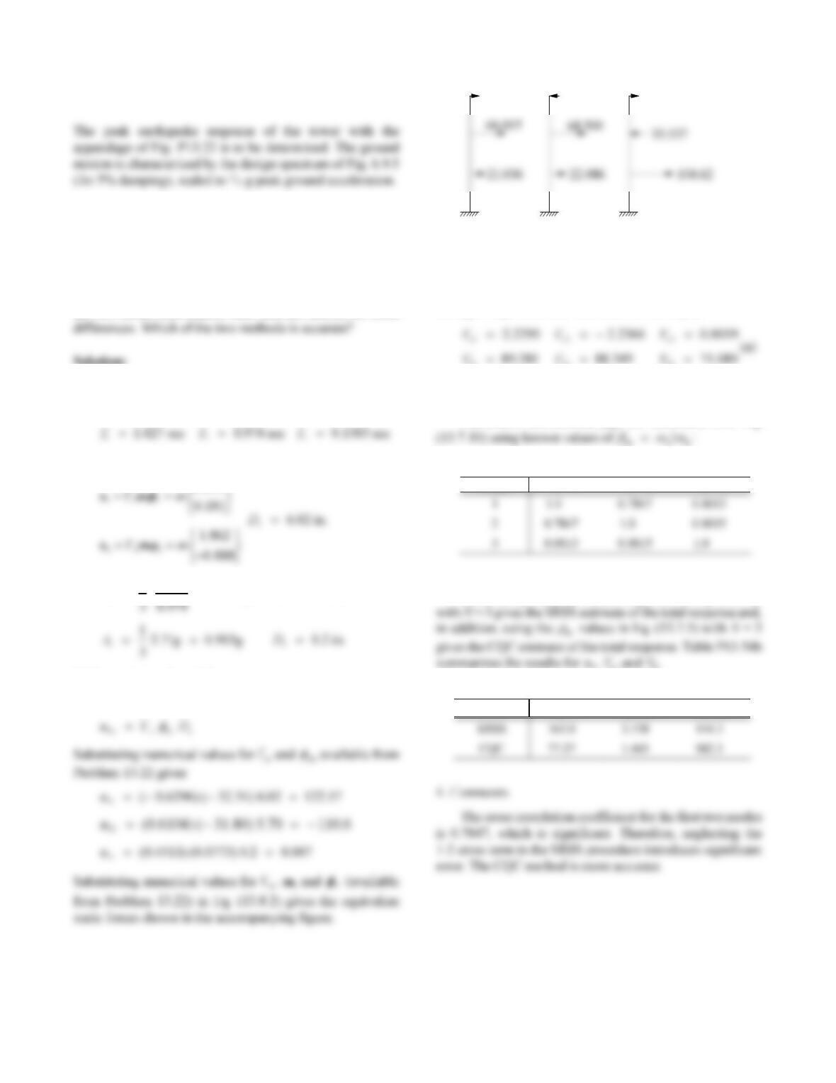
119

Problem 13.54

(a) Using the SRSS and CQC modal combination rules,

calculate the peak values of the following response

quantities: (i) the displacement of the appendage mass, (ii)

the shear force at the base of the appendage, and (iii) the

shear force at the base of the tower.

(b) Comment on the differences between the results from

the two modal combination rules and the reasons for these

Solution:

1. Determine design spectrum ordinates.

From Problem 13.22,

For these

T

n, the design spectrum of Fig. 6.9.5 gives

0.259



2

11.80g 0.616g

V

A

25.70 in.D

2. Determine peak modal responses.

The appendage displacement is



Static analysis of the structure subjected to forces fn

gives the peak value of modal response

r

n. These results for

the appendage shear and base shear are (in kips):

12 3

bb b

3. Combine modal responses.

Correlation coefficients,



Table P13.54a: Correlation coefficients



in

Mode, i n = 1 n = 2 n = 3

Substituting the peak modal responses in Eq. (13.7.3)

a, and

b.

Table P13.54b

u3, in.

V

a, kips

V

b, kips

f1

2.2295

2.2366

f2

0.0059

f3

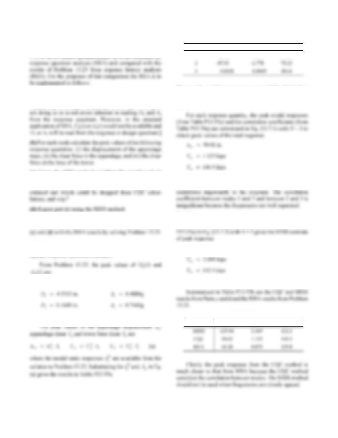
120

Problem 13.55

The peak response of the tower with the appendage of Fig.

(a) Determine the spectral ordinates Dn and An for the nth-

mode SDF system as the peak values of Dn(t) and An(t),

respectively, determined in part (a) of Problem 13.23. [We

(c) Using the CQC method, combine the modal peak to

determine the peak value of each of the response quantities

of part (b). Which of the modal correlation terms must be

(e) Comment on the accuracy of the CQC and SRSS modal

combination rules by comparing the RSA results from parts

Solution:

D

A

n()

14.3641 in.D 10.4237gA

Part b: Peak modal responses.

V

A

Table P13.55a

Mode, n u3, in.

V

a, kips

V

b, kips

1 88.90 1.619 64.83

These peak modal responses are essentially identical to

those determined in Problem 13.23 by RHA.

Part c

The cross-correlation coefficient for the first two modes

is 0.7847 (see Problem 13.54), which is significant and

Part d

Substituting the peak modal responses (from Table

3125.04 in.

o

u

Part e: Comments.

Table P13.55b

uo3, in.

V

ao , kips

V

bo , kips

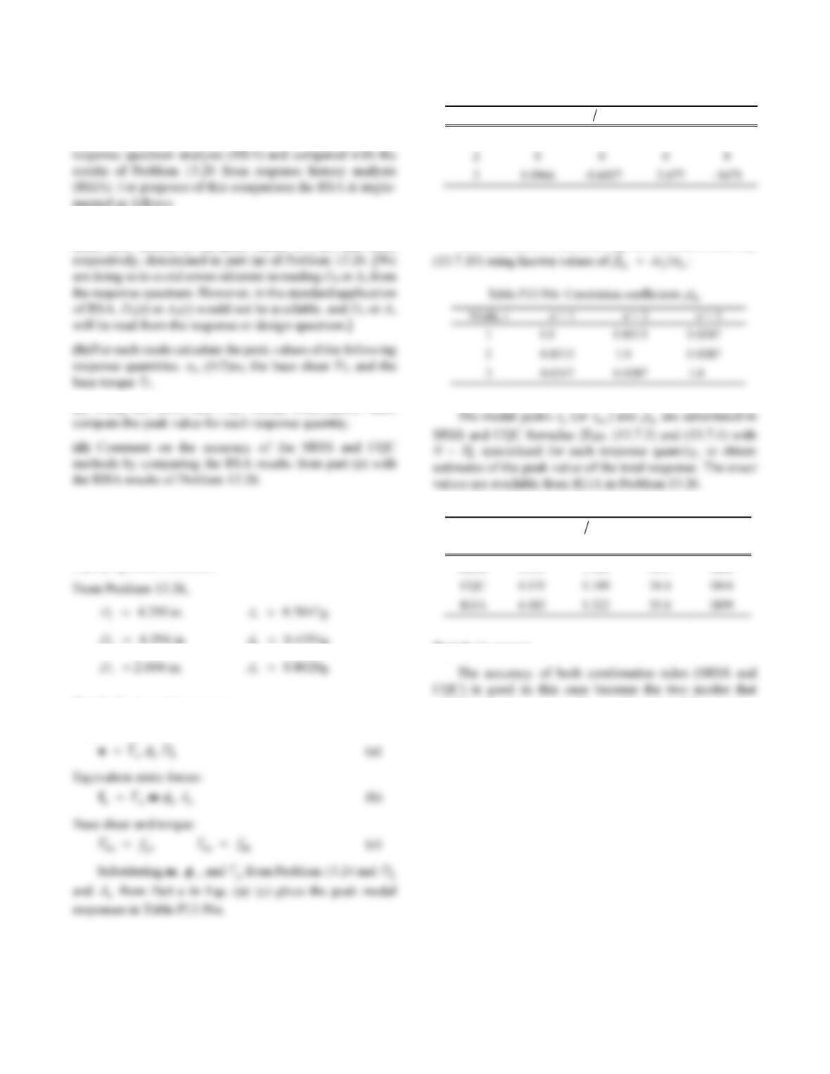
121

Problem 13.56

The peak response of the one-story, unsymmetric-plan

system of Fig. P13.24 with ζn = 5% is to be estimated by

mented as follows.

(a) Determine the spectral ordinates Dn and An for the nth-

mode SDF system as the peak values of Dn(t) and An(t),

(c) Using the SRSS and CQC modal combination rules,

r



Solution:

From Problem 13.24, m, n



, and n are available.

Part a: Spectral ordinates.

24.354 in.D 20.4354gA

Part b: Peak modal responses.

Displacements:

A



T





D

A

Table P13.56a

Mode, n uy ()bu2



V

b

T

b

1 4.132 0.9931 34.21 822.2

Part c

The correlation coefficients



in are calculated from Eq.

Table P13.56c

uy,

in.

()bu2



,

in.

V

b,

kips

T

b,

kip–ft

SRSS 4.133 1.162 34.3 1862

Part d: Comments.

contribute to the response have well separated frequencies.

Both methods are similarly accurate in this case.

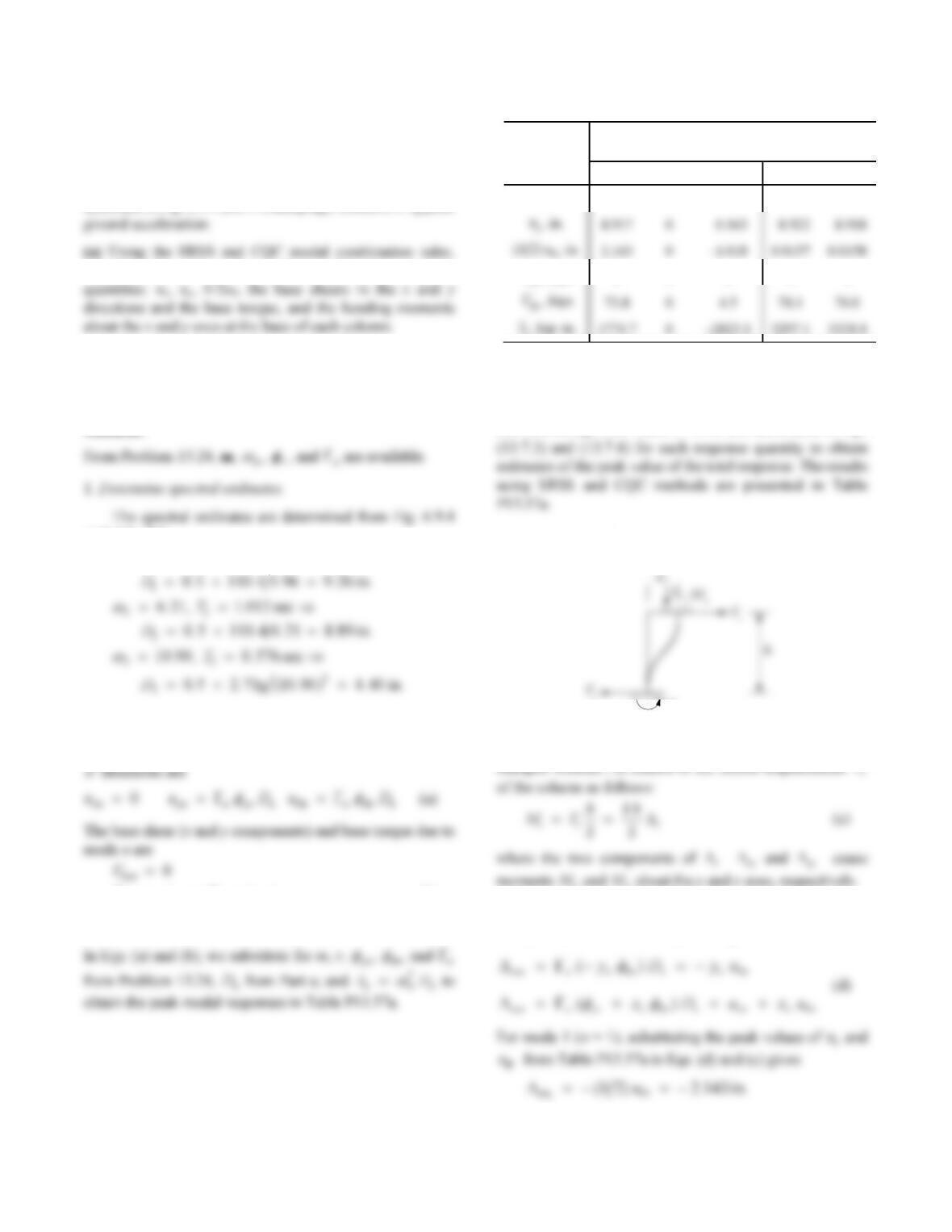
122

Problem 13.57

Determine the peak response of the one-story, unsymmetric-

plan system of Fig. P13.24 to ground motion along the

y-direction. The excitation is characterized by the design

spectrum of Fig. 6.9.5 (for 5% damping), scaled to 0.5g peak

calculate the peak values of the following response

(b) Comment on the differences between the results from

the two modal combination rules and the reasons for these

differences. Which of the two methods is accurate?

Solution:

scaled by 0.5:



1596.,

T

11 054. sec 

D



T

D

2. Determine peak modal responses.

Due to mode n, the peak displacements in the x, y, and

x

D



D



V

M

V

f

m

A

byn yn n yn n





(b)

Tf mr A

bn nnnn







()

2





D

x

Table P13.57a

Response Peak modal responses Peak total

response

n = 1 n = 2 n = 3 CQC SRSS

u

x

, in. 0 0 0 0 0

V

bx , kips 0 0 0 0 0

b, kip–in. 1774.7 0 –2823.1 3297.1 3334.4

3. Combine peak modal responses.

The modal peaks (from Part b) and correlation

coefficients



4. Determine bending moments in columns.

i

M

i

The bending moment

M

i at the ends of a clamped-

clamped column i is related to the lateral displacement



y and

x

We illustrate the procedure for column a in Fig. P13.24.

The peak modal values of



ax and ay are

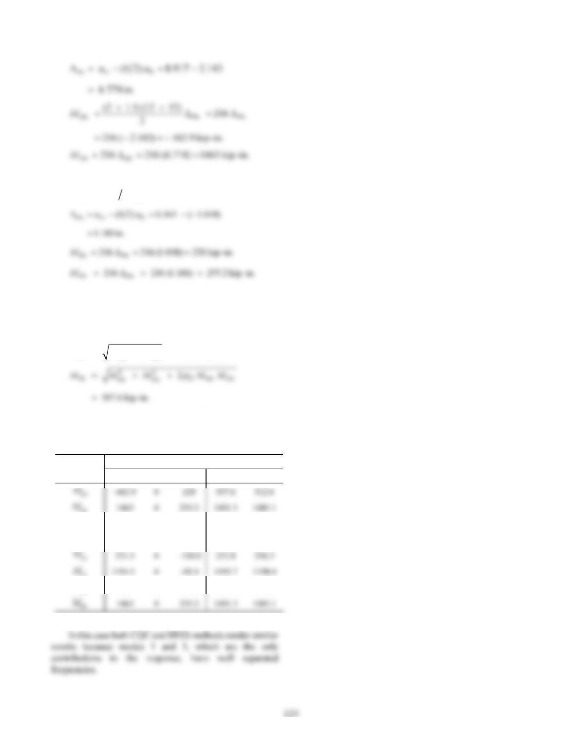
The computations for mode 3 proceed similarly:

33

(2) 1.018in.

ax bu



 

Specializing Eqs. (13.7.3) and (13.7.4) for the SRSS

and CQC methods to response

M

ay, and substituting for

1

ay

M

and 3

ay

M

(from above) and 13 0.0247



 (from

Problem 13.56) gives

13

22

512.5 kip–in.

ay ay

ay

MMM

Similar computations lead to Table P13.57b for

M

ax and

bending moments in other columns.

Table P13.57b: Column moments in kip–in.

Response Peak modal responses Peak total response

n = 1 n = 2 n = 3 CQC SRSS

M

by –231.5 0 110.0 253.8 256.3

M

bx 1194.5 0 –92.4 1195.7 1198.0

M

dy 462.9 0 –220 507.6 512.6

M

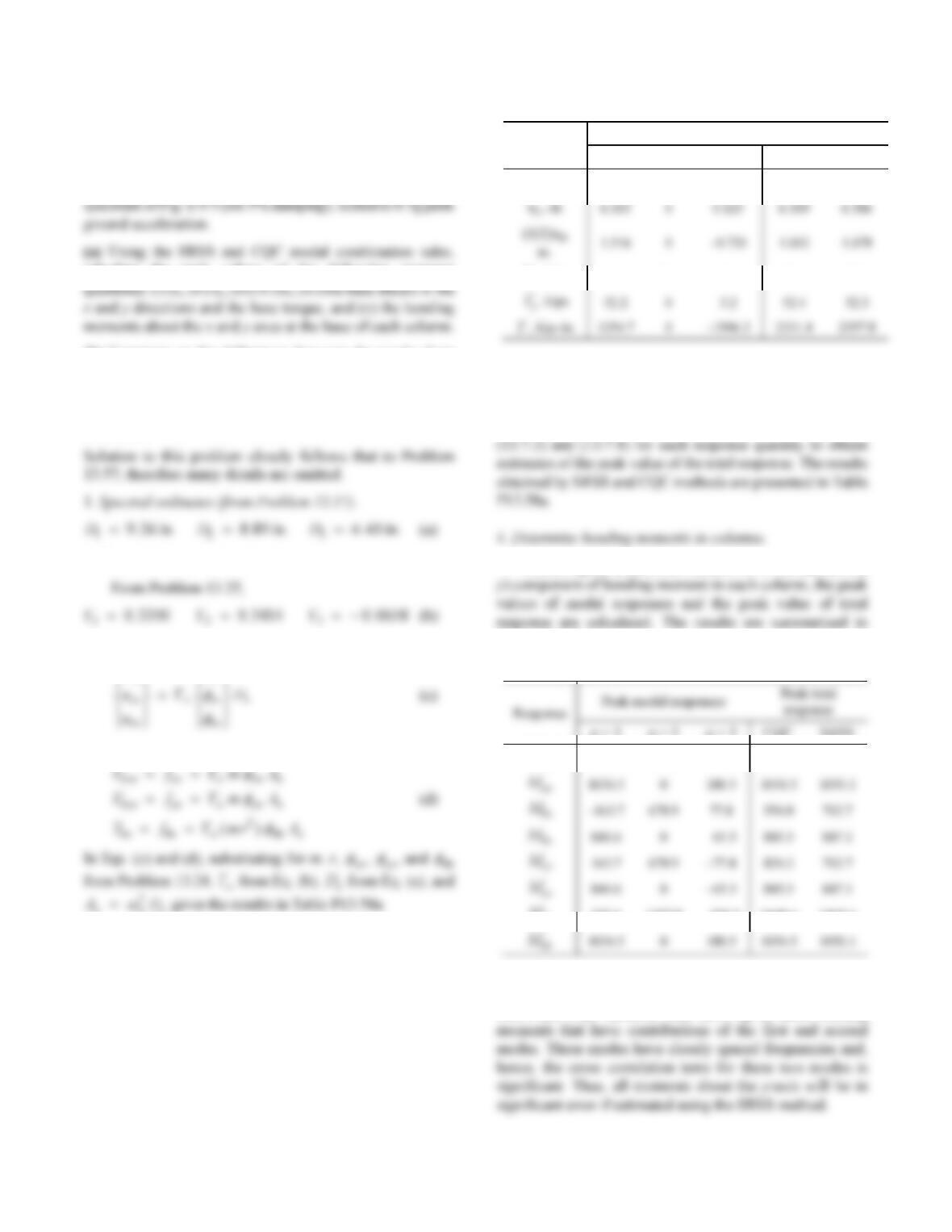
124

Problem 13.58

Determine the peak response of the one-story, unsymmetric-

plan system of Fig. P13.24 to ground motion along the

diagonal d–b. The excitation is characterized by the design

calculate the peak values of the following response

(b) Comment on the differences between the results from

the two modal combination rules and the reasons for these

differences. Which of the two methods is accurate?

Solution:

2. Determine peak modal responses.

Displacements:

xn xn

u



 

Base forces:

x



V

A

x

M

nnn

Table P13.58a

Response Peak modal responses Peak total response

n = 1 n = 2 n = 3 CQC SRSS

ux, in. 0 6.286 0 6.286 6.286

V

x

, kips 0 56.6 0 56.6 56.6

3. Combine peak modal responses.

The modal peaks (from Table P13.58a) and correlation

coefficients



in (from Table P13.56b) are substituted in Eqs.

Following the solution of Problem 13.57 for each (x and

Table P13.58b.

Table P13.58b: Column moments in kip–in.

n = 1 n = 2 n = 3 CQC SRSS

M

ay –327.4 1357.8 155.5 1108.1 1405.4

M

dy 327.4 1357.8 –155.5 1648.4 1405.4

It is interesting to note that the differences between the

SRSS and CQC methods only show up in those bending

125