221
WHAT’S NEW IN THE SIXTH EDITION:
There are no major changes in this chapter.
LEARNING OBJECTIVES:
By the end of this chapter, students should understand:
➢ what items are included in a firm’s costs of production.
➢ the relationship between short-run and long-run costs.
CONTEXT AND PURPOSE:
Chapter 13 is the first chapter in a five-chapter sequence dealing with firm behavior and the organization
of industry. It is important that students become comfortable with the material in Chapter 13 because
Chapters 14 through 17 are based on the concepts developed in Chapter 13. To be more specific,
KEY POINTS:
• The goal of firms is to maximize profit, which equals total revenue minus total cost.
THE COSTS OF PRODUCTION
13
222 ❖ Chapter 13/The Costs of Production
• When analyzing a firm’s behavior, it is important to include all the opportunity costs of production.
Some of the opportunity costs, such as the wages a firm pays its workers, are explicit. Other
opportunity costs, such as the wages the firm owner gives up by working in the firm rather than
taking another job, are implicit. Economic profit takes both explicit and implicit costs into account,
whereas accounting profits consider only explicit costs.
• From a firm’s total cost, two related measures of cost are derived. Average total cost is total cost
divided by the quantity of output. Marginal cost is the amount by which total cost rises if output
increases by one unit.
CHAPTER OUTLINE:
I. What Are Costs?
A. Total Revenue, Total Cost, and Profit
1. The goal of a firm is to maximize profit.
This is an extremely important chapter, and it is critical that students have an
understanding of the important principles developed here in order to follow the
material presented in the next several chapters. Do not be surprised at the number
of students who are unfamiliar with such seemingly simple concepts as revenue,
costs, and profits.
Point out to students that it is possible for firm owners to have different goals, but
the one motive that makes the most accurate prediction about how firm managers
Chapter 13/The Costs of Production ❖ 223
2. Definition of total revenue: the amount a firm receives for the sale of its output.
3. Definition of total cost: the market value of the inputs a firm uses in production.
B. Costs as Opportunity Costs
1. Principle #2: The cost of something is what you give up to get it.
2. The costs of producing an item must include all of the opportunity costs of inputs used in
production.
3. Total opportunity costs include both implicit and explicit costs.
a. Definition of explicit costs: input costs that require an outlay of money by the
firm.
costs.
C. The Cost of Capital as an Opportunity Cost
1. The opportunity cost of financial capital is an important cost to include in any analysis of firm
performance.
Total Revenue = Price Quantity
Students rarely have trouble understanding the concept of explicit costs. However,
224 ❖ Chapter 13/The Costs of Production
D. Economic Profit versus Accounting Profit
1. Figure 1 highlights the differences in the ways in which economists and accountants calculate
profit.
4. If implicit costs are greater than zero, accounting profit will always exceed economic profit.
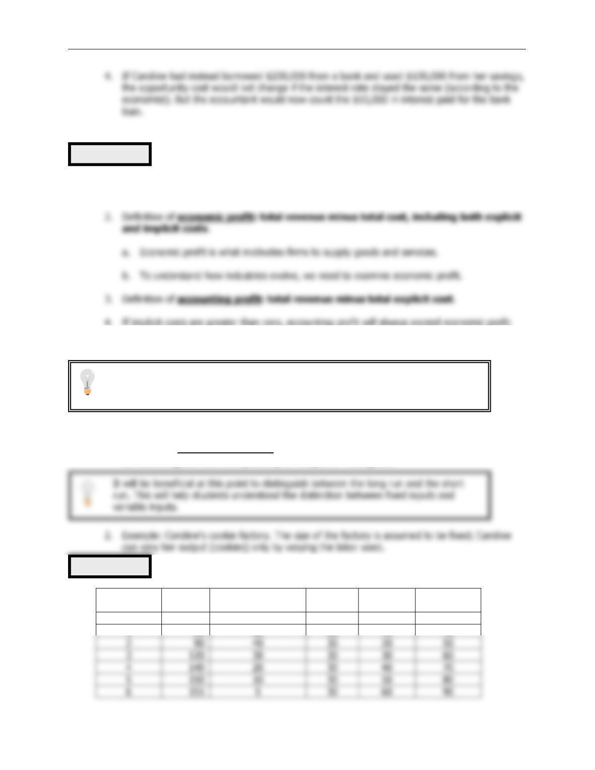
II. Production and Costs
A. The Production Function
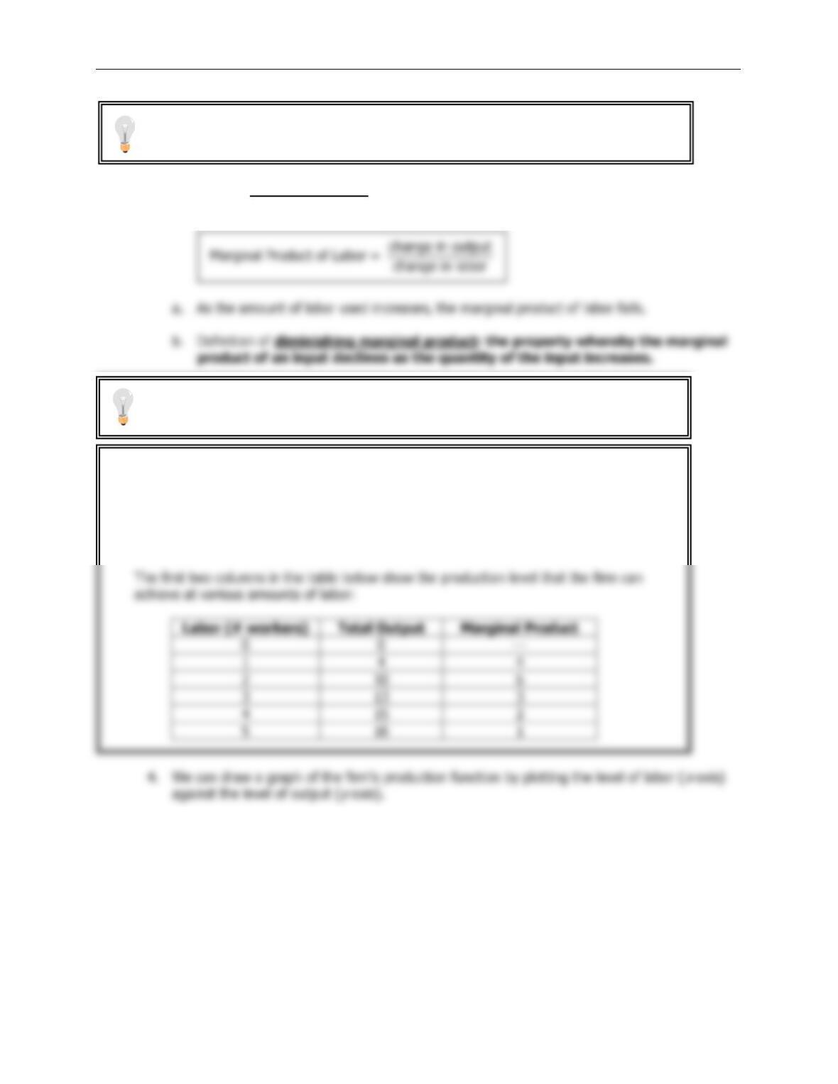
1. Definition of production function: the relationship between quantity of inputs used
to make a good and the quantity of output of that good.
Number of
Workers
Output
Marginal Product
of Labor
Cost of
Factory
Cost of
Workers
Total Cost
of Inputs
0
0
—
$30
$0
$30
1
50
50
30
10
40
2
90
40
30
20
50
3
120
30
30
30
60
5
150
10
30
50
80
6
155
30
60
90
Figure 1
Table 1
You may want to give students a handout that summarizes the definitions and
provides them an opportunity to practice the calculations in this chapter. (See the
alternative classroom examples.)
Chapter 13/The Costs of Production ❖ 225
3. Definition of marginal product: the increase in output that arises from an additional
unit of input.
Go through this table, column by column. Make sure that students understand the
calculations involved.
Point out that diminishing marginal returns is a result of fixed inputs and, therefore is
a short-run phenomenon.
ALTERNATIVE CLASSROOM EXAMPLE:
Consider the short-run production of a small firm that makes sweaters. These sweaters are
made using a combination of labor and knitting machines. In the short run, the firm has
signed a lease to rent one machine. Therefore, in the short run, the firm cannot vary the
amount of knitting machines it uses. However, the firm can vary the amount of labor it
employs.
226 ❖ Chapter 13/The Costs of Production
B. From the Production Function to the Total-Cost Curve
1. We can draw a graph of the firm’s total cost curve by plotting the level of output (
x
-axis)
against the total cost of producing that output (
y
-axis).
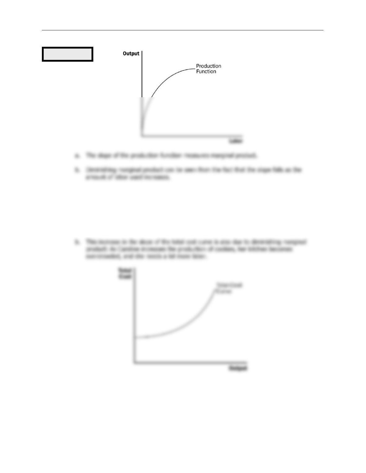
a. The total cost curve gets steeper and steeper as output rises.
Figure 2
Chapter 13/The Costs of Production ❖ 227
III. The Various Measures of Cost
A. Example: Conrad’s Coffee Shop
B. Fixed and Variable Costs
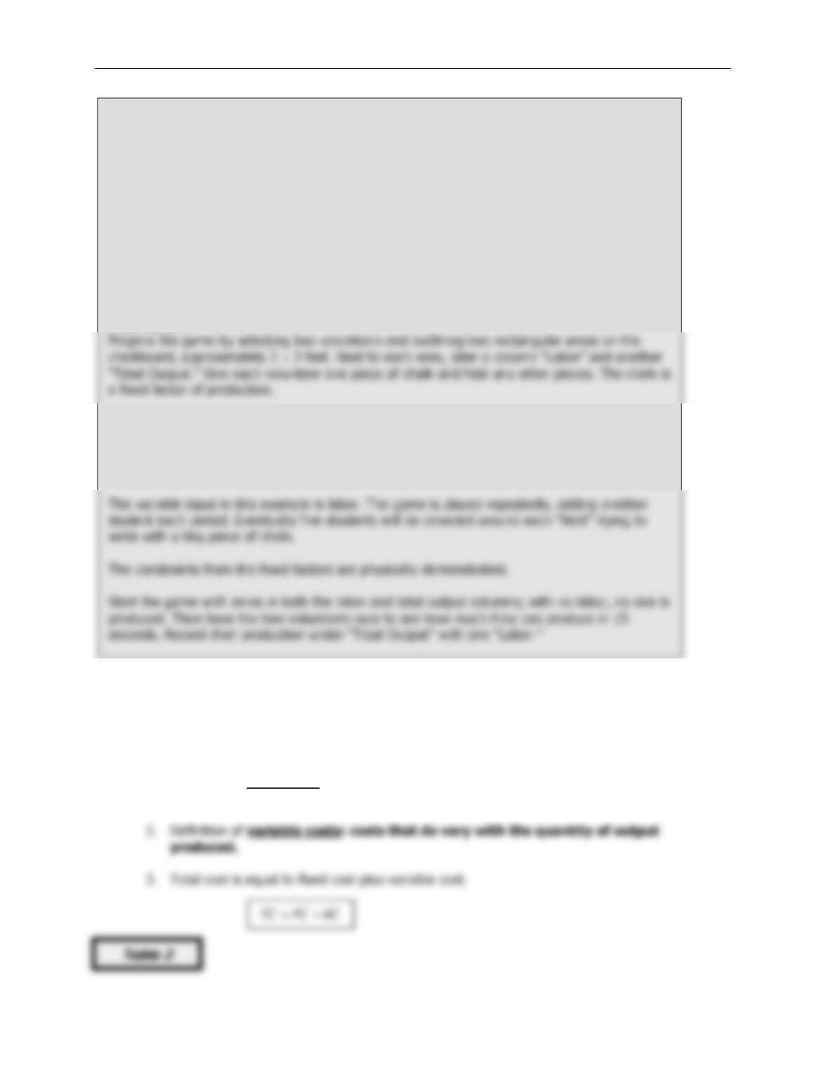
1. Definition of fixed costs: costs that do not vary with the quantity of output
produced.
Activity 1—Growing Rice on a Chalkboard
Type: In-class demonstration
Topics: Diminishing returns and increasing costs
Materials needed: Chalkboard and chalk
Time: 25 minutes
Class limitations: Works in classes with more than 15 students
Purpose
Students often have difficulty understanding why diminishing returns exist in short-run
production. This activity vividly demonstrates how fixed factors constrain the returns to
variable inputs. Then the cause of increasing marginal cost is obvious.
Instructions
The volunteers are farmers and the outlined areas are their farm fields. They produce rice by
writing the word “RICE” in large letters inside their own field. The letters need to be at least
three inches high. They want to produce as much rice as possible in each 15-second time
period.
228 ❖ Chapter 13/The Costs of Production
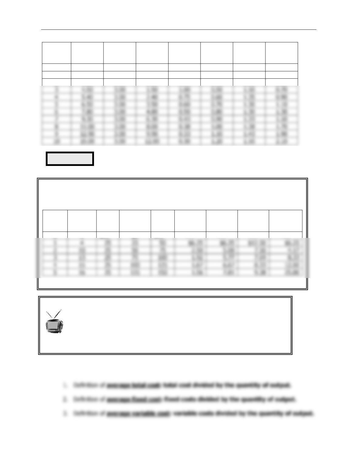
Output
Total
Cost
Fixed
Cost
Variable
Cost
Average
Fixed
Cost
Average
Variable
Cost
Average
Total
Cost
Marginal
Cost
0
$3.00
$3.00
$0
—
—
—
—
1
3.30
3.00
0.30
$3.00
$0.30
$3.30
$0.30
2
3.80
3.00
0.80
1.50
0.40
1.90
0.50
C. Average and Marginal Cost
ALTERNATIVE CLASSROOM EXAMPLE:
Consider the sweater manufacturer (described earlier). The firm is currently renting one machine
for $25 per day. Each worker is also paid $25 per day.
Labor
Output
Fixed
Cost
Variable
Cost
Total
Cost
Average
Fixed
Cost
Average
Variable
Cost
Average
Total
Cost
Marginal
Cost
0
0
$25
$0
$25
—-
—-
—-
—-
1
4
25
2
50
3
75
4
5
Figure 3
Seinfeld, “The Bottle Deposit.”
(Season 7, 3:14-4:37; 5:36-5:55; 12:48-
15:38; 26:29-26:56.) Kramer and Newman hatch a scheme to arbitrage bottles
from New York, where the deposit is 5 cents, to Michigan, where the deposit is 10
cents. They can’t figure out how to make the costs work; gas is too expensive
(variable costs), and there’s too much overhead (fixed costs of tolls, permits, etc.)
with using a semi to haul the bottles in volume. Finally, they hatch a scheme to use a
mail truck, which lowers their variable and fixed costs to zero.
3
4.50
3.00
1.50
1.00
0.50
1.50
0.70
4
5.40
3.00
2.40
0.75
0.60
1.35
0.90
5
6.50
3.00
3.50
0.60
0.70
1.30
1.10
6
7.80
3.00
4.80
0.50
0.80
1.30
1.30
7
9.30
3.00
6.30
0.43
0.90
1.33
1.50
8
3.00
8.00
0.38
1.00
1.38
1.70
9
3.00
9.90
0.33
1.10
1.43
1.90
3.00
0.30
1.20
1.50
2.10
Chapter 13/The Costs of Production ❖ 229
4. Definition of marginal cost: the increase in total cost that arises from an extra unit
of production.
D. Cost Curves and Their Shapes
1. Rising Marginal Cost
a. This occurs because of diminishing marginal product.
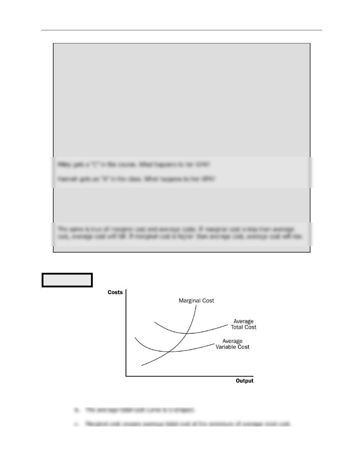
2. U-Shaped Average Total Cost
a. Average total cost is the sum of average fixed cost and average variable cost.
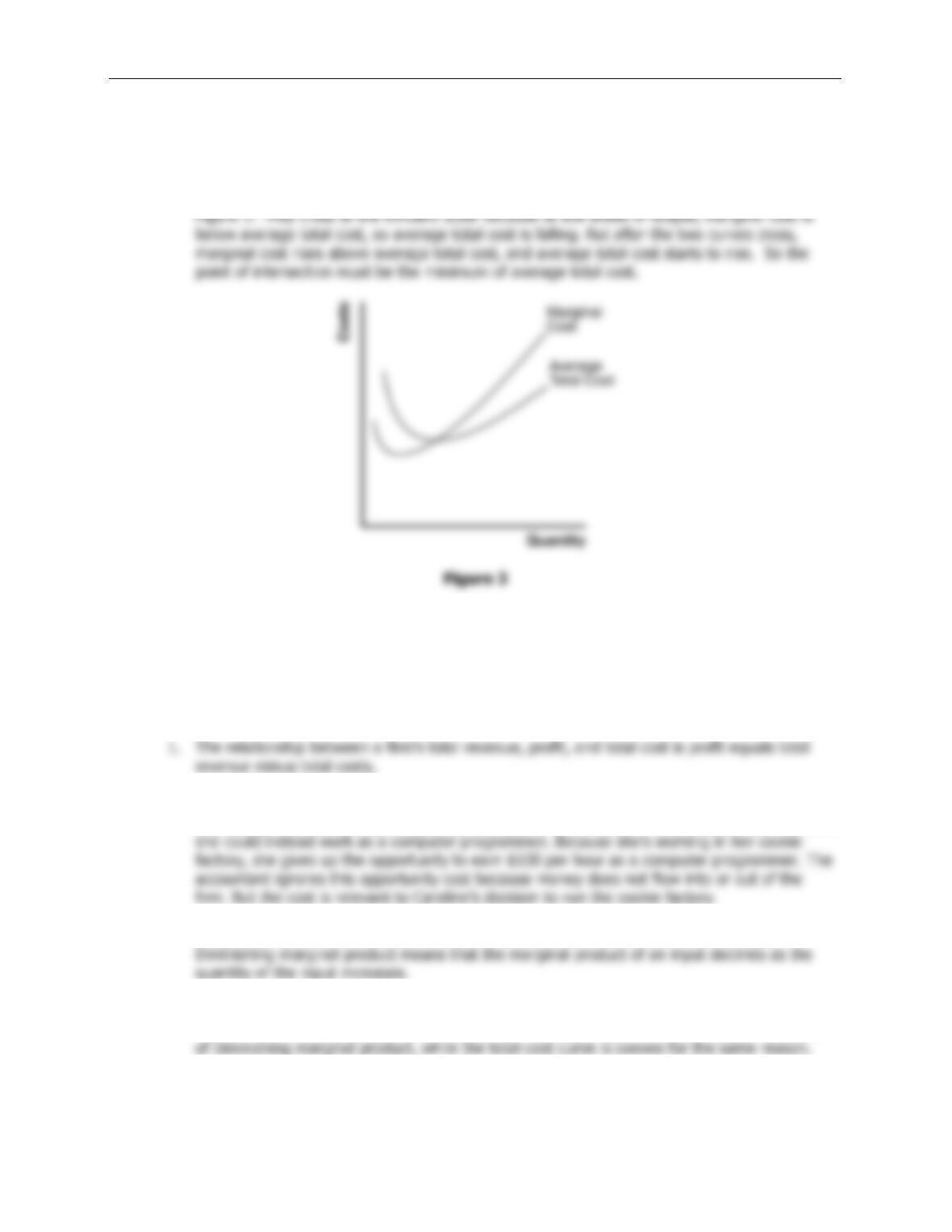
3. The Relationship between Marginal Cost and Average Total Cost
a. Whenever marginal cost is less than average total cost, average total cost is falling.
Whenever marginal cost is greater than average total cost, average total cost is rising.
b. The marginal-cost curve crosses the average-total-cost curve at minimum average total
cost (the efficient scale).
;;
TC VC FC
ATC AVC AFC
Q Q Q
= = =
ATC AFC AVC
=+
Figure 4
230 ❖ Chapter 13/The Costs of Production
4. Typical Cost Curves
a. Marginal cost eventually rises with output.
Activity 2—Average and Marginal Grades
Type: In-class demonstration
Topics: Relationship between marginal and average cost
Materials needed: None
Time: 5 minutes
Class limitations: Works in any size class
Purpose
This quick exercise uses an analogy to illustrate to students that they already know the
relation between marginal values and averages.
Instructions
Tell the class that two twins (Miley and Hannah) are enrolled in Principles of Economics. They
each had a “B” average (GPA = 3.0) before taking the class.
Common Answers and Points for Discussion
Students will likely know that Miley will have a lower GPA and Hannah a higher GPA. A
“marginal” grade lower than the average will pull down the average. A “marginal” grade
higher than the average will increase the average.
Figure 5
Chapter 13/The Costs of Production ❖ 231
IV. Costs in the Short Run and in the Long Run
A. The division of total costs into fixed and variable costs will vary from firm to firm.
B. Some costs are fixed in the short run, but all are variable in the long run.
1. For example, in the long run a firm could choose the size of its factory.
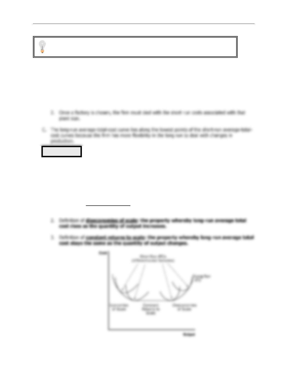
D. The long-run average-total-cost curve is typically U-shaped, but is much flatter than a typical
short-run average-total-cost curve.
E. The length of time for a firm to get to the long run will depend on the firm involved.
F. Economies and Diseconomies of Scale
1. Definition of economies of scale: the property whereby long-run average total cost
falls as the quantity of output increases.
Figure 6
Emphasize that these cost curves include ALL costs for the resources needed to
produce the good. Thus, both explicit costs and implicit costs are included.
232 ❖ Chapter 13/The Costs of Production
4.
FYI: Lessons from a Pin Factory
SOLUTIONS TO TEXT PROBLEMS:
Quick Quizzes
1. Farmer McDonald’s opportunity cost is $300, consisting of 10 hours of lessons at $20 an hour
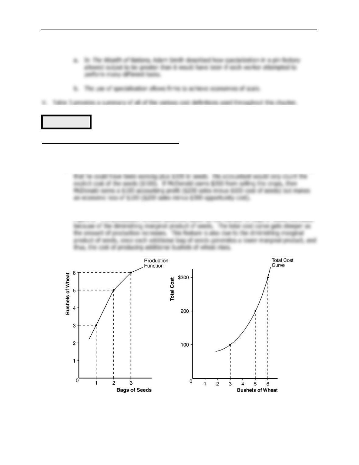
2. Farmer Jones’s production function is shown in Figure 1 and his total-cost curve is shown in
Figure 2. The production function becomes flatter as the number of bags of seeds increases
Figure 1 Figure 2
Table 3
Chapter 13/The Costs of Production ❖ 233
3. The average total cost of producing 5 cars is $250,000/5 = $50,000. Since total cost rose
from $225,000 to $250,000 when output increased from 4 to 5, the marginal cost of the fifth
car is $25,000.
The marginal-cost curve and the average-total-cost curve for a typical firm are shown in
4. The long-run average total cost of producing 9 planes is $9 million/9 = $1 million. The long–
run average total cost of producing 10 planes is $9.5 million/10 = $0.95 million. Since the
long-run average total cost declines as the number of planes increases, Boeing exhibits
economies of scale.
Questions for Review
2. An accountant would not count the owner’s opportunity cost of alternative employment as an
accounting cost. An example is given in the text in which Caroline runs a cookie business, but
3. Marginal product is the increase in output that arises from an additional unit of input.
4. Figure 4 shows a production function that exhibits diminishing marginal product of labor.
Figure 5 shows the associated total-cost curve. The production function is concave because
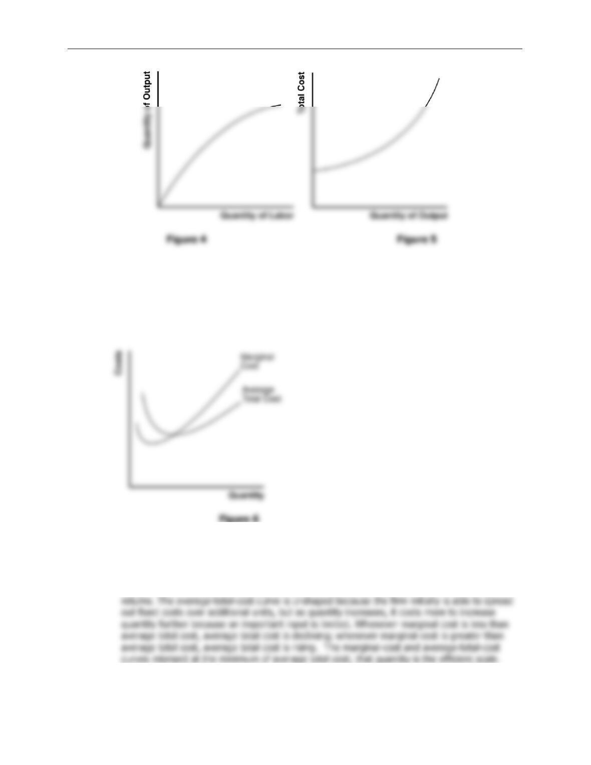
234 ❖ Chapter 13/The Costs of Production
5. Total cost consists of the costs of all inputs needed to produce a given quantity of output. It
includes fixed costs and variable costs. Average total cost is the cost of a typical unit of
output and is equal to total cost divided by the quantity produced. Marginal cost is the cost
of producing an additional unit of output and is equal to the change in total cost divided by
the change in quantity. An additional relation between average total cost and marginal cost is
that whenever marginal cost is less than average total cost, average total cost is declining;
whenever marginal cost is greater than average total cost, average total cost is rising.
Figure 6
6. Figure 6 shows the marginal-cost curve and the average-total-cost curve for a typical firm. It
has three main features: (1) marginal cost is rising; (2) average total cost is U-shaped; and
(3) whenever marginal cost is less than average total cost, average total cost is declining;
whenever marginal cost is greater than average total cost, average total cost is rising.
Marginal cost is rising for output greater than a certain quantity because of diminishing
Chapter 13/The Costs of Production ❖ 235
7. In the long run, a firm can adjust the factors of production that are fixed in the short run; for
8. Economies of scale exist when long-run average total cost falls as the quantity of output
Problems and Applications
2. a. The opportunity cost of something is what must be given up to acquire it.
b. The opportunity cost of running the hardware store is $550,000, consisting of $500,000
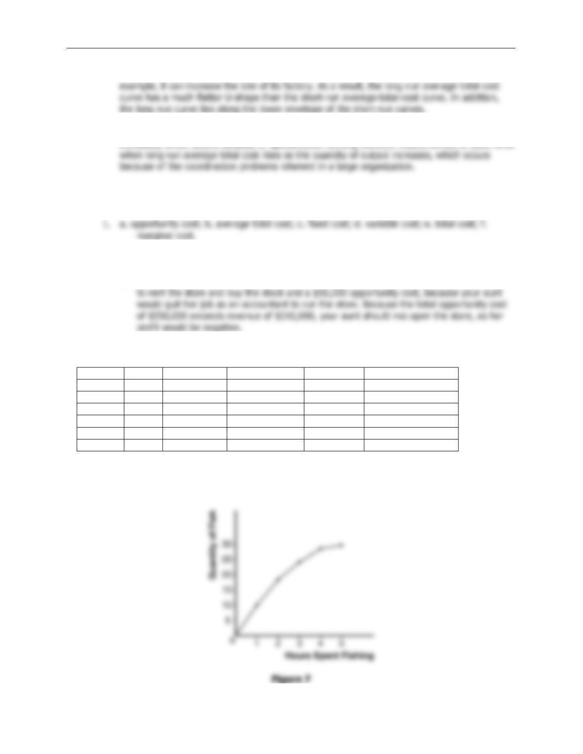
3. a. The following table shows the marginal product of each hour spent fishing:
Hours
Fish
Fixed Cost
Variable Cost
Total Cost
Marginal Product
0
0
$10
$0
$10
—
1
10
10
5
15
10
2
18
10
10
20
8
3
24
10
15
25
6
4
28
10
20
30
4
5
30
10
25
25
2
b. Figure 7 graphs the fisherman’s production function. The production function becomes
flatter as the number of hours spent fishing increases, illustrating diminishing marginal
product.
236 ❖ Chapter 13/The Costs of Production
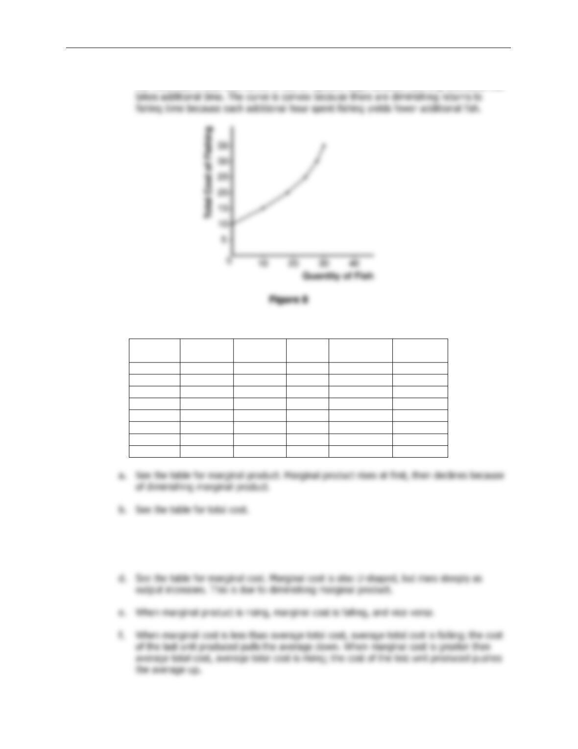
c. The table shows the fixed cost, variable cost, and total cost of fishing. Figure 8 shows
the fisherman’s total-cost curve. It has an upward slope because catching additional fish
4. Here is the table of costs:
Workers
Output
Marginal
Product
Total
Cost
Average
Total Cost
Marginal
Cost
0
0
—
$200
—
—
1
20
20
300
$15.00
$5.00
2
50
30
400
8.00
3.33
3
90
40
500
5.56
2.50
4
120
30
600
5.00
3.33
5
140
20
700
5.00
5.00
6
150
10
800
5.33
10.00
7
155
5
900
5.81
20.00
c. See the table for average total cost. Average total cost is U-shaped. When quantity is
low, average total cost declines as quantity rises; when quantity is high, average total
cost rises as quantity rises.
Chapter 13/The Costs of Production ❖ 237
5. At an output level of 600 players, total cost is $180,000 (600 × $300). The total cost of
6. a. The fixed cost is $300, because fixed cost equals total cost minus variable cost. At an
output of zero, the only costs are fixed cost.
b.
Quantity
Total
Cost
Variable
Cost
Marginal Cost
(using total cost)
Marginal Cost
(using variable cost)
0
$300
$0
—
—
1
350
50
$50
$50
2
390
90
3
420
120
4
450
150
5
490
190
6
540
240
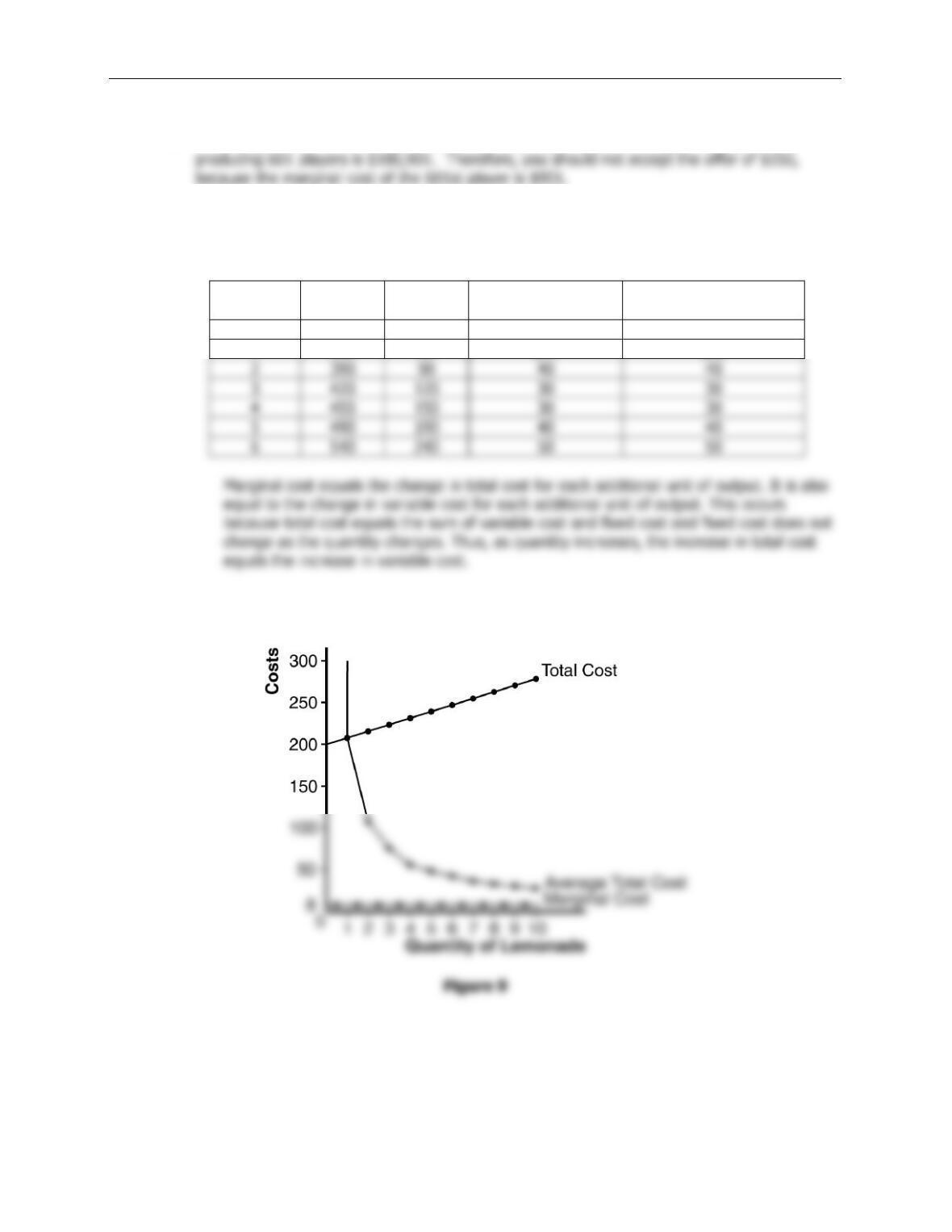
7. a. The fixed cost of setting up the lemonade stand is $200. The variable cost per cup is
$0.50.
238 ❖ Chapter 13/The Costs of Production
b. The following table shows total cost, average total cost, and marginal cost. These are
plotted in Figure 9.
Quantity
(gallons)
Total Cost
Average Total Cost
Marginal Cost
0
$200
—
—
1
208
$208
$8
8. The following table illustrates average fixed cost (
AFC
), average variable cost (
AVC
), and
average total cost (
ATC
) for each quantity. The efficient scale is 4 houses per month,
because that minimizes average total cost.
Quantity
Variable
Cost
Fixed
Cost
Total
Cost
Average
Fixed Cost
Average
Variable Cost
Average
Total Cost
0
$0
$200
$200
—
—
—
1
10
2
20
10
3
40
5
32
6
7
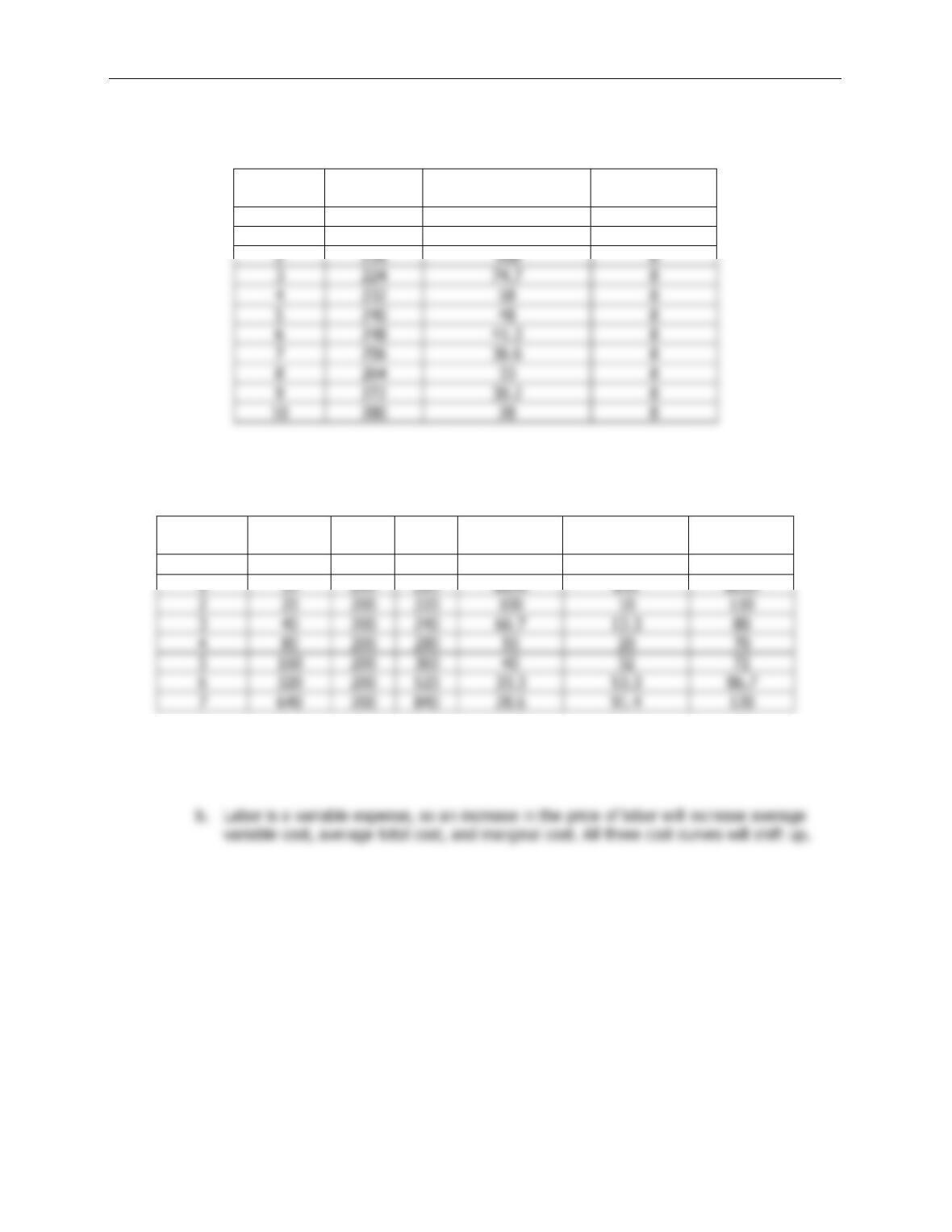
9. a. Since capital is fixed in the short run, the cost of capital is a fixed cost. Therefore, only
average total cost will be affected by a rise in the price of capital. Average variable cost
and marginal cost will remain the same. The average-total-cost curve will shift up.
2
216
3
224
4
232
5
240
6
248
7
256
8
264
9
272
280
Chapter 13/The Costs of Production ❖ 239
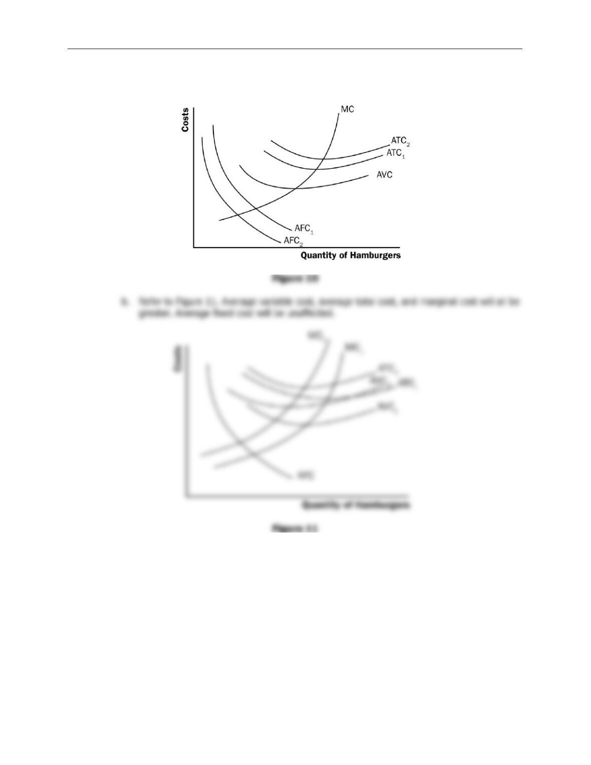
10. a. The lump-sum tax causes an increase in fixed cost. Therefore, as Figure 10 shows, only
average fixed cost and average total cost will be affected.
240 ❖ Chapter 13/The Costs of Production
11. a. The following table shows average variable cost (
AVC
), average total cost (
ATC
), and
marginal cost (
MC
) for each quantity.
Quantity
Variable
Cost
Total
Cost
Average
Variable Cost
Average
Total Cost
Marginal
Cost
0
$0
$30
—
—
—
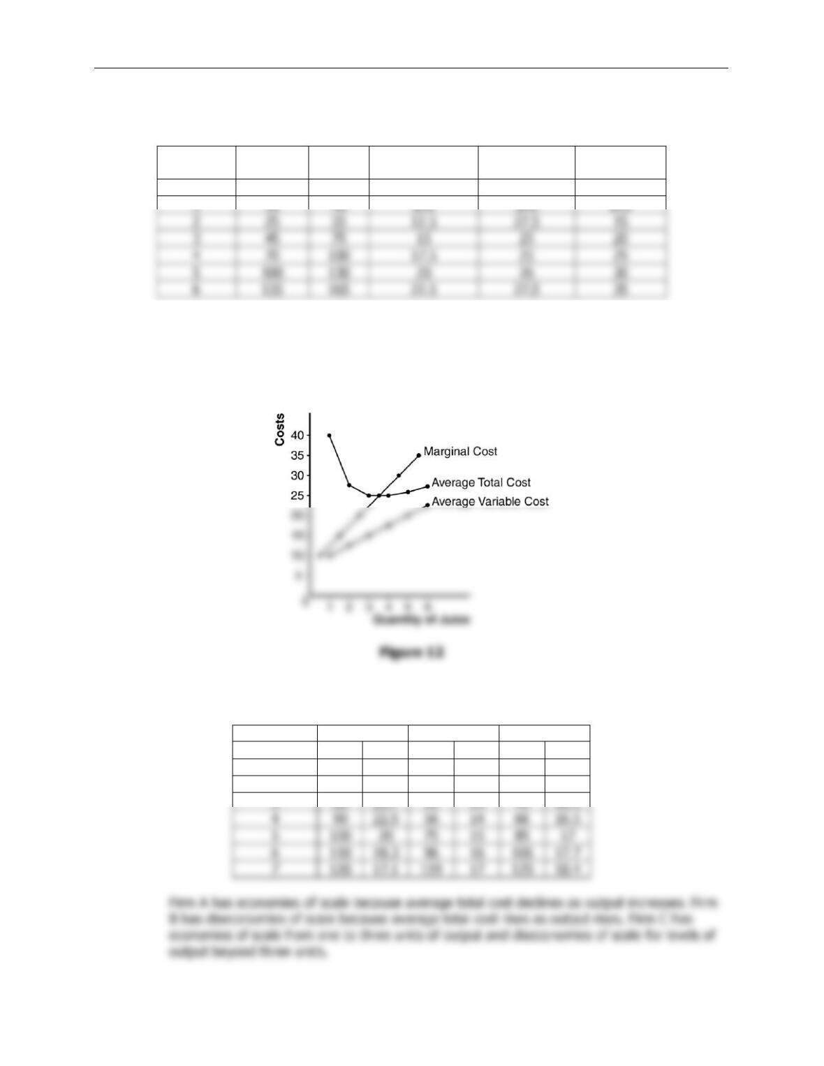
b. Figure 12 shows the three curves. The marginal-cost curve is below the average-total-
cost curve when output is less than four and average total cost is declining. The
marginal-cost curve is above the average-total-cost curve when output is above four and
average total cost is rising. The marginal-cost curve lies above the average-variable-cost
curve.
12. The following table shows quantity (
Q
), total cost (
TC
), and average total cost (
ATC
) for the
three firms:
Firm A
Firm B
Firm C
Quantity
TC
ATC
TC
ATC
TC
ATC
1
$60
$60
$11
$11
$21
$21
2
70
35
24
12
34
17
3
80
39
13
49
4
90
56
14
66
5
100
20
75
15
85
17
6
110
96
16
106
7
120
119
17
129
1
10
2
25
45
70
100
130
165