126
Problem 13.59
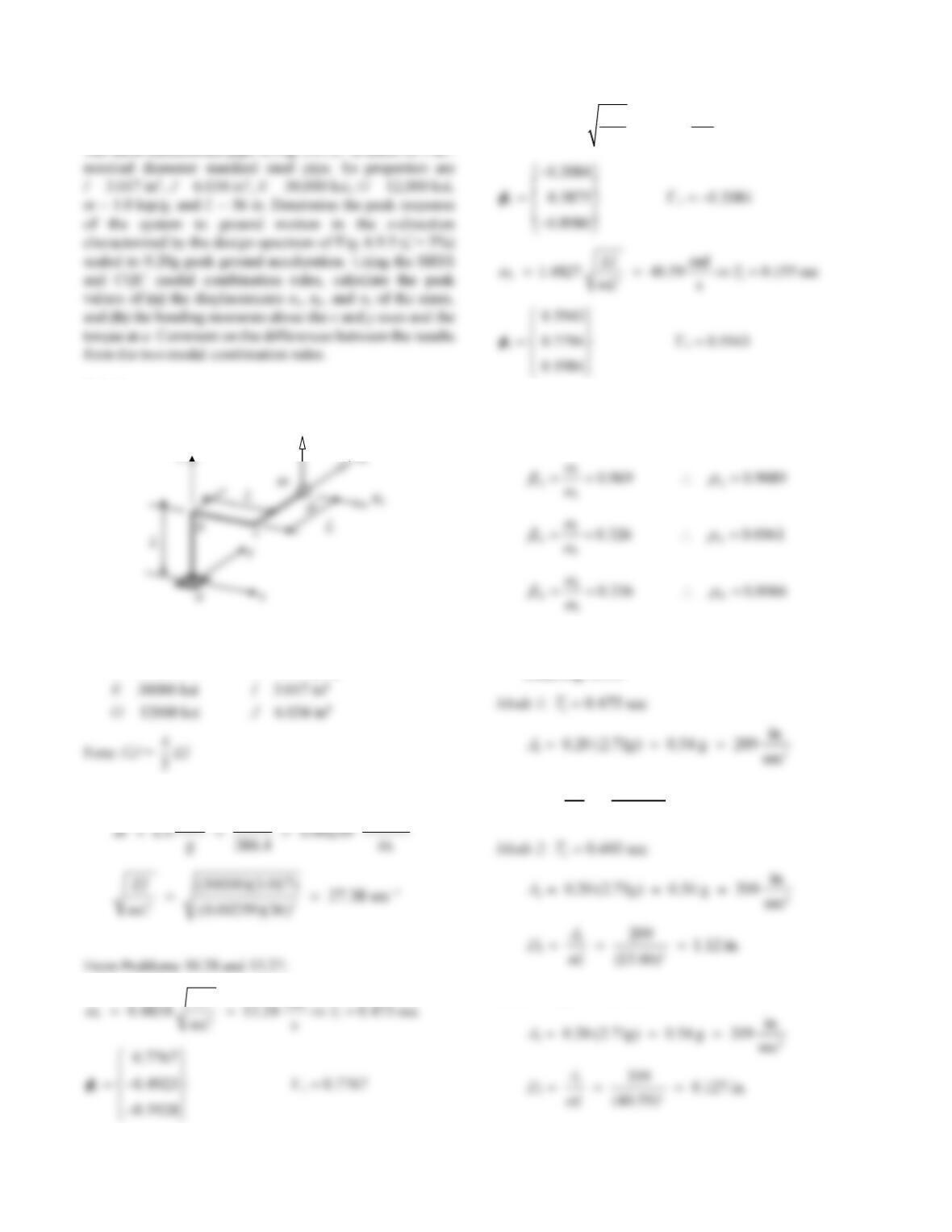
The three-dimensional pipe of Fig. P13.27 is made of 3-in.–
Solution:
y
x
1. Data.
L = 36 in. m = 1.0 kips/g
2. Natural frequencies and modes.
2
kips 1.0 k sec
rad
EI T
22
3
rad
0.4990 13.66 0.460 sec
s
EI T
mL
3. Determine correlation coefficients.
Use Eq. (13.7.10) to compute ij
for
= 0.05:
4. Determine spectral ordinates.
From Fig. 6.9.5:
1
122
1
209 1.20 in.
(13.24)
A
D
Mode 3: 30.155 secT
z
uz
uy
127
5. Determine peak modal displacements.
7212.0
7767.0
0488.0
2084.0
0150.0
1984.0
6. Combine peak modal displacements.
Using Eqs. (13.7.3) and (13.7.4), the SRSS and CQC
Displacement SRSS rule
(in.)
CQC rule
(in.)
7. Determine peak modal responses.
Problem 13.27 as:
mLmLmLM
st
xn
3453.0,2679.0,0773.0
Substituting numerical values for st
yn
st
xn MM ,, st
n
T, and An
in Eq. (b) gives:
1
19.234 k in.
T
8. Combine peak modal responses.
Using Eqs. (13.7.3) and (13.7.4), the SRSS and CQC
9. Comments.
Modes 1 and 2 are strongly correlated with each other
(
12 = 0.9089), but weakly correlated with mode 3.
Consequently, significant differences between the SRSS
and CQC estimates should result only when both modes 1
significantly. The effect of modal correlation is less
pronounced for the other displacements and responses either
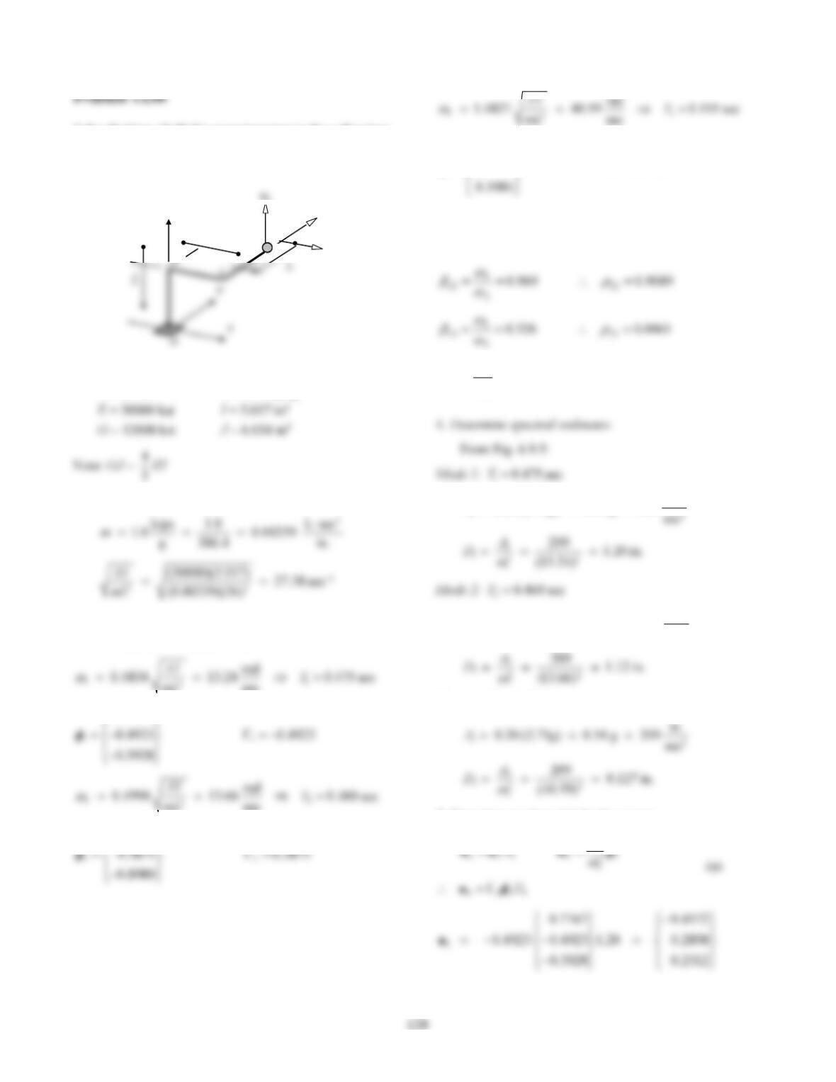
Solve Problem 13.59 for ground motion in the y-direction.
Solution:
L
y
x
1. Data.
L = 36 in. m = 1.0 kips/g
2. Natural frequencies and modes.
From Problems 10.28 and 13.28:
sec
0.7767
mL
sec
0.2084
mL
33
0.5943
0.7794 0.7794
3. Determine correlation coefficients.
Use Eq. (13.7.10) to compute ij
for
= 0.05:
0066.0336.0
23
3
2
23
12
in.
0.20 (2.71g) 0.54 g 209 sec
A
22
in.
0.20 (2.71g) 0.54 g 209 sec
A
Mode 3: 30.155 secT
5. Determine peak modal displacements.
n
st st
L
m
z
d
uy
ux
129
1685.0
0906.0
12.1
3975.0
2084.0
3875.0
2
u
6. Combine peak modal displacements.
Using Eqs. (13.7.3) and (13.7.4), the SRSS and CQC
Displacement SRSS rule
(in.)
CQC rule
(in.)
7. Determine peak modal responses.
Problem 13.28 as:
mLmLmLM
st
xn
4528.0,4982.0,0490.0
Substituting numerical values for st
yn
st
xn MM ,, st
n
T, and An
in Eq. (b) gives:
1
0.956 k in.
x
M
1
11.235 k in.
y
M
8. Combine peak modal responses.
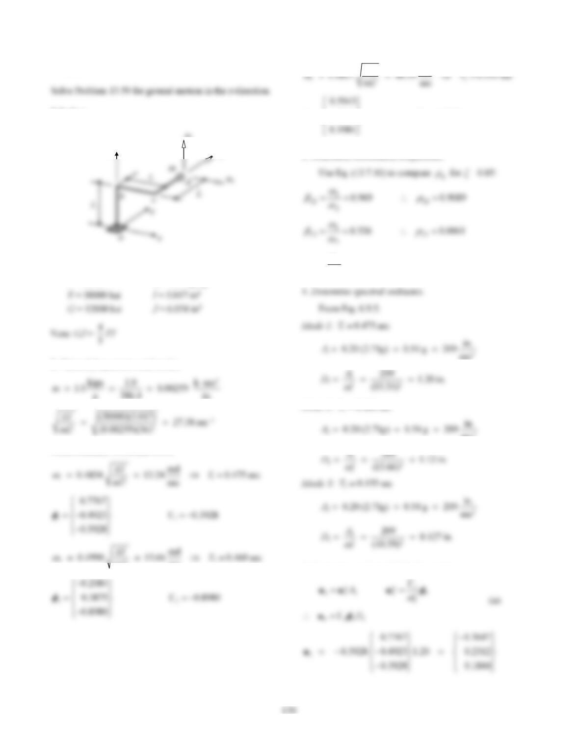
calculated. These estimates are summarized in the following
table.
9. Comments.
Modes 1 and 2 are strongly correlated with each other
contribute significantly to the total response. Examining the
above results, we see that this is the case. The SRSS and
CQC estimates for the displacements uy and uz and responses
Problem 13.61
Solution:
y
x
1. Data.
L = 36 in. m = 1.0 kips/g
2. Natural frequencies and modes.
From Problems 10.28 and 13.29:
3
sec
mL
33
rad
0.7794 0.1984
EI T
3. Determine correlation coefficients.
0066.0336.0
23
3
2
23
Mode 2: 20.460 secT
5. Determine peak modal displacements.
z
uz
uy
131
3905.0
2100.0
12.1
3975.0
2084.0
8980.0
u
6. Combine peak modal displacements.
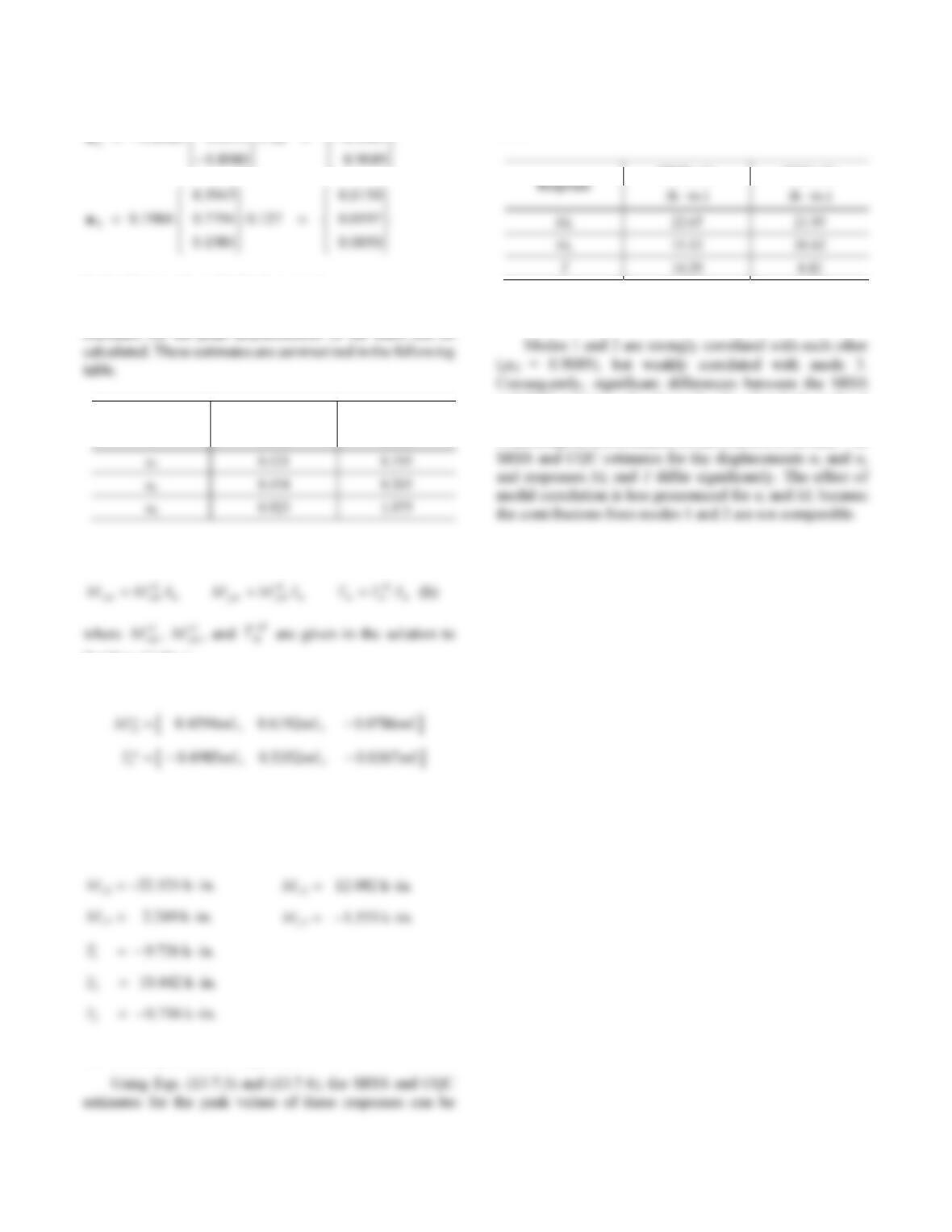
Using Eqs. (13.7.3) and (13.7.4), the SRSS and CQC
estimates for the peak displacements of the mass can be
Displacement SRSS rule
(in.)
CQC rule
(in.)
7. Determine peak modal responses.
Problem 13.29 as:
0.0391 , 1.1544 , 0.1153
st
xn
MmLmLmL
Substituting numerical values for st
yn
st
xn MM ,, st
n
T, and An
in Eq. (b) gives:
1
0.763 k in.
x
M
1
8.963 k in.
y
M
8. Combine peak modal responses.
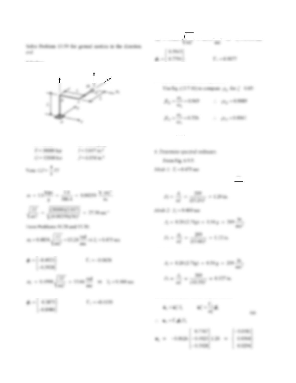
calculated. These estimates are summarized in the following
table.
CQC rule
9. Comments.
and CQC estimates should result only when both modes 1
and 2 contribute significantly to the total response.
Examining the above results, we see that this is the case. The
132
Problem 13.62
Solution:
y
x
1. Data.
L = 36 in. m = 1.0 kips/g
2. Natural frequencies and modes.
0.7767
0.2084
rad
0.1984
EI T
3. Determine correlation coefficients.
0066.0336.0
23
3
2
23
12
in.
0.20 (2.71g) 0.54 g 209 sec
A
Mode 3: 30.155 secT
5. Determine peak modal displacements.
z
uz
uy
133
4182.0
1805.0
0971.0
12.1
8980.0
3975.0
2084.0
4150.0
2
u
0686.0
5943.0
table.
Displacement SRSS rule
(in.)
CQC rule
(in.)
7. Determine peak modal responses.
Substituting numerical values for st
yn
st
xn MM ,, st
n
T, and An
in Eq. (b) gives:
1
0.122 k in.
x
M
1
1.428 k in.
y
M
8. Combine peak modal responses.
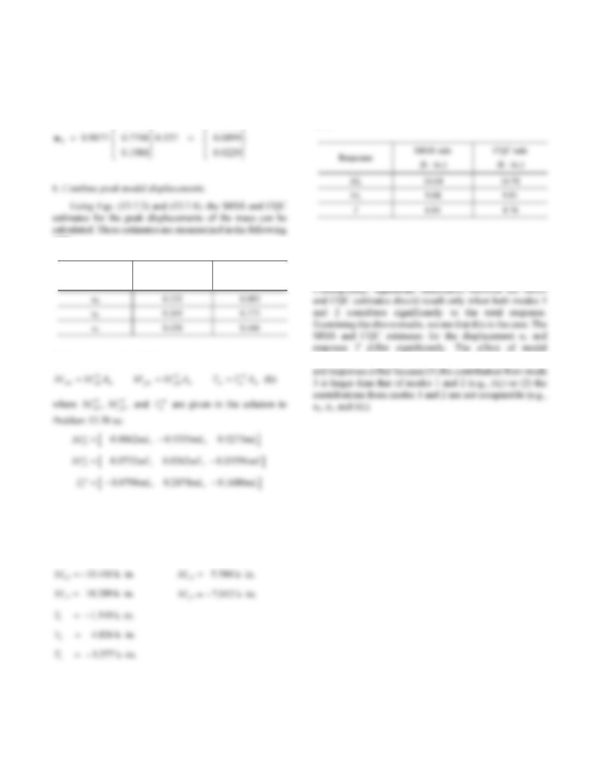
Using Eqs. (13.7.3) and (13.7.4), the SRSS and CQC
estimates for the peak values of these responses can be
calculated. These estimates are summarized in the following
table.
9. Comments.
Modes 1 and 2 are strongly correlated with each other
(
12 = 0.9089), but weakly correlated with mode 3.
correlation is less pronounced for the other displacements
134
Problem 13.63
For the structure and ground motion defined in Problem
Solution:
1. Data.
L = 36 in. m = 1.0 kips/g
2
kips 1.0 k sec
1.0 0.00259
m
From Problems 10.28 and 13.27:
11
rad
0.4834 13.24 0.475 sec
EI T
rad
EI T
33
3
rad
1.4827 40.59 0.155 sec
sec
EI T
mL
3. Determine correlation coefficients.
Use Eq. (13.7.10) to compute ij
for
= 0.05:
4. Determine spectral ordinates.
From Fig. 6.9.5:
Mode 2: 20.460 secT
Mode 3: 30.155 secT
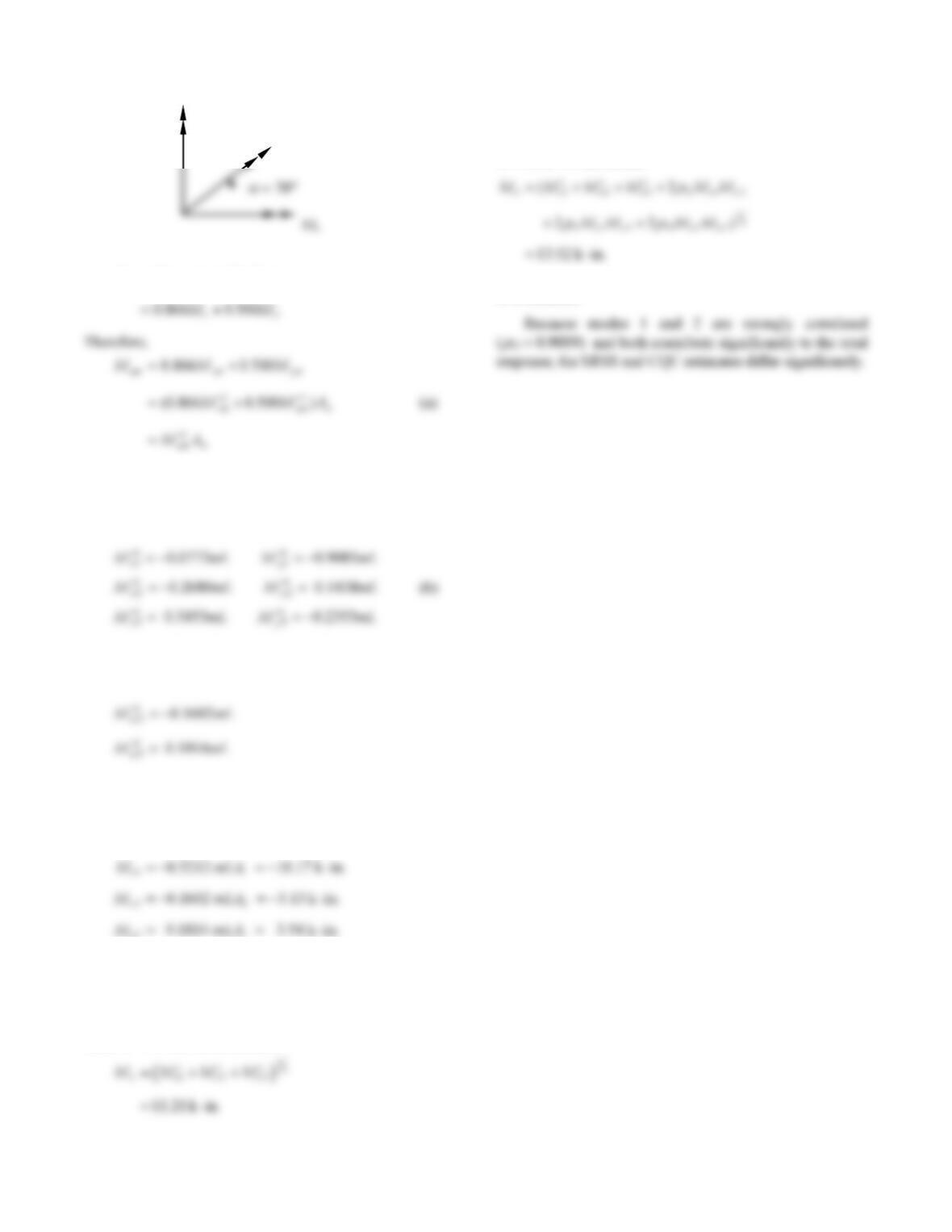
5. Determine modal static responses for M
uz
uy
135
cos sin
xy
MM M
Thus,
0.866 0.500
s
tstst
nxnyn
M
MM
where st
xn
M and
s
t
yn
M
are
given in the solution to Problem 13.27:
Equation (a), after substituting Eq. (b) becomes
mLM
st
5212.0
1
6. Determine peak modal responses M
n.
The peak values, M
n, of the modal contributions M
n(t)
to response M
are determined next
7. Combine peak modal responses.
(a) SRSS rule
Using Eq. (13.7.3), the SRSS estimate for the peak
value of M
can be calculated:
(b) CQC rule
Using Eq. (13.7.4), the CQC estimate for the peak value
of M
can be calculated :
8. Comments.
M
M
y
M
136
Problem 13.64
Solution:
y
x
L = 36 in. m = 1.0 kips/g
E = 30000 ksi I = 3.017 in.4
1
(30000)(3.017) 27.38 sec
EI
From Problems 10.28 and 13.28:
sec
mL
33
rad
0.7794 0.7794
EI T
3. Determine correlation coefficients.
Use Eq. (13.7.10) to compute ij
for
= 0.05:
4. Determine spectral ordinates.
Mode 2: 20.460 secT
Mode 3: 30.155 secT
5. Determine modal static responses for M
L
m
z
uz
uy
ux
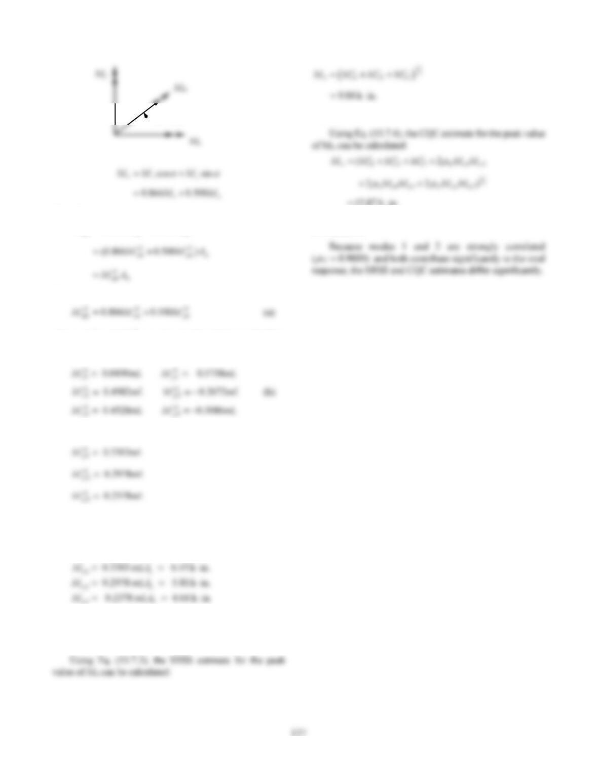
Therefore,
ynxnn
MMM
500.0866.0
Thus,
where st
xn
M and st
yn
M are given in the solution to Problem
13.28:
Equation (a), after substituting Eq. (b) becomes
6. Determine peak modal responses M
n.
The peak values, M
n, of the modal contributions M
n(t)
to response M
are determined next
7. Combine peak modal responses.
(a) SRSS rule
(b) CQC rule
12.87 k in.
8. Comments.
138
Problem 13.65
y
x
1. Data.
Note: GJ = 5
4EI
1
(30000)(3.017) 27.38 s
EI
0.2084
rad
1.4827 40.59 0.155 sec
EI T
3. Determine correlation coefficients.
Use Eq. (13.7.10) to compute ij
for
= 0.05:
0066.0336.0
23
3
2
23
Mode 1: 10.475 secT
Mode 2: 20.460 secT
Mode 3: 30.155 secT
5. Determine modal static responses for M
.
L
m
z
d
uy
ux
139
Therefore,
ynxnn
MMM
500.0866.0
Thus,
13.29:
mLMmLM
st
y
st
x
4593.00392.0
11
Equation (a), after substituting Eq. (b) becomes
mLM
st
2635.0
1
6. Determine peak modal responses M
n.
The peak values, M
n, of the modal contributions M
n(t)
to response M
are determined next
11
0.2635 5.14 k in.
MmLA
7. Combine peak modal responses.
(a) SRSS rule
(b) CQC rule
8. Comments.
Because modes 1 and 2 are strongly correlated
140
Problem 13.66
Solve Problem 13.63 for ground motion in the direction
L
y
x
L = 36 in. m = 1.0 kips/g
E = 30000 ksi I = 3.017 in.4
From Problems 10.28 and 13:30:
0.2084
0.5943
3. Determine correlation coefficients.
Use Eq. (13.7.10) to compute ij
for
= 0.05:
4. Determine spectral ordinates.
5. Determine modal static responses for M
.
L
m
z
uz
uy
ux
Therefore,
ynxnn
MMM
500.0866.0
Thus,
where st
xn
M and st
yn
M are given in the solution to Problem
13.30:
mLMmLM
st
y
st
x
0731.00062.0
11
Equation (a), after substituting Eq. (b) becomes
mLM
st
0420.0
1
6. Determine peak modal responses M
n.
The peak values, M
n, of the modal contributions M
n(t)
to response M
are determined next
11
0.0420 0.82 k in.
MmLA
7. Combine peak modal responses.
(a) SRSS rule
(b) CQC rule
8. Comments.
142
Problem 13.67
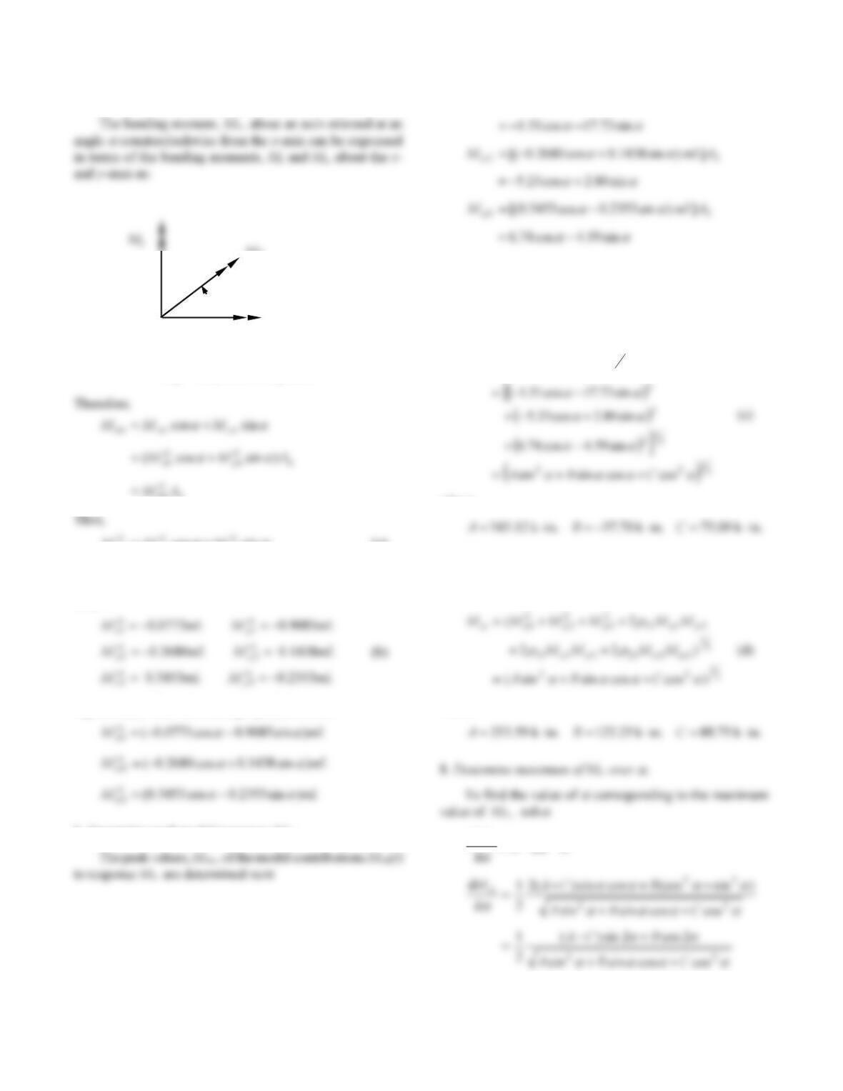
(a) For the structure defined in Problem 13.59 and ground
(b) Compute the maximum value of the peak bending
L
y
x
1. Data.
L = 36 in. m = 1.0 kips/g
E = 30000 ksi I = 3.017 in.4
2. Natural frequencies and modes.
0.7767
22
3
rad
0.4990 13.66 0.460 sec
sec
EI T
mL
3. Determine correlation coefficients.
Use Eq. (13.7.10) to compute ij
for
= 0.05:
0066.0336.0
23
3
2
23
4. Determine spectral ordinates.
12
in.
0.20 (2.71g) 0.54 g 209 sec
A
Mode 3: 30.155 secT
L
m
z
uy
ux
143
5. Determine modal static responses for M
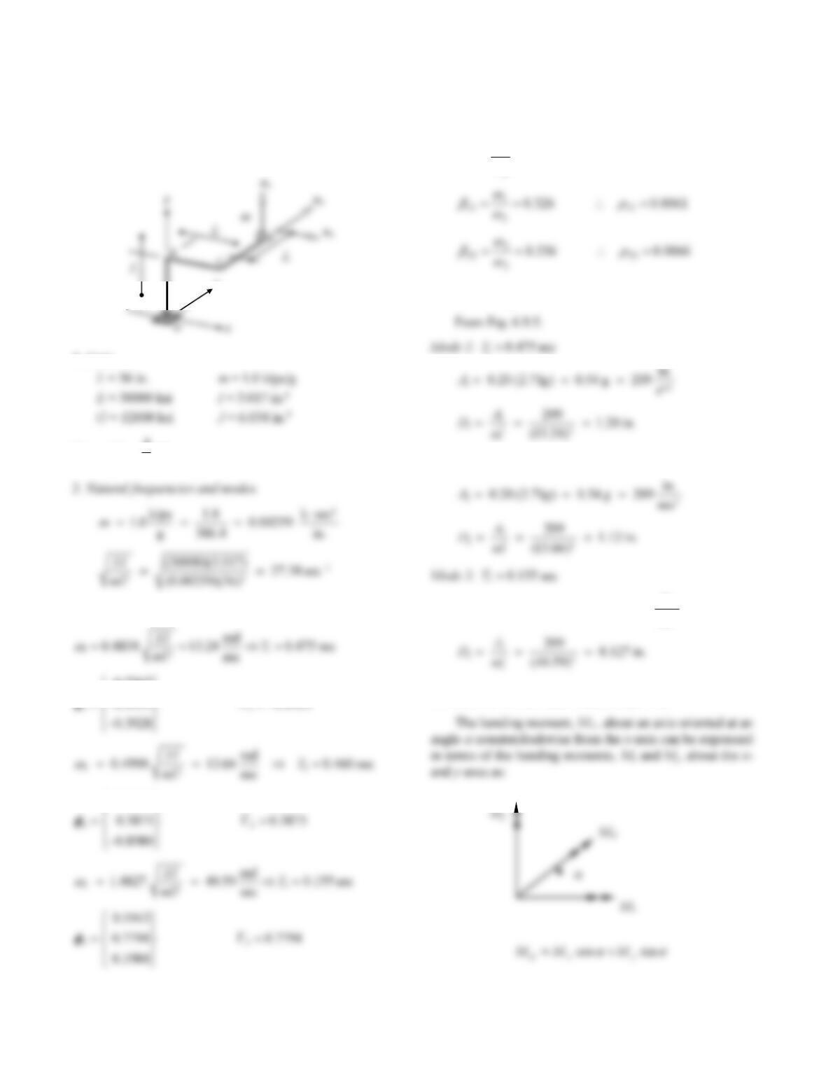
sincos yx MMM
n
n
sincos st
yn
xn
nMMM (a)
where st
xn
M and st
yn
M are given in the solution to Problem
13.27:
Equation (a), after substituting Eq. (b) becomes
6. Determine peak modal responses M
n..
])sin9085.0cos0773.0[(
11
AmLM
7. Combine peak modal responses.
(a) SRSS rule
Using Eq. (13.7.3), the SRSS estimate for the peak
value of M
can be calculated:
2
1
2
3
2
2
2
1
MMMM
where
(b) CQC rule
Using Eq. (13.7.4), the CQC estimate for the peak value
of M
can be calculated:
where
for0
d
M
M
x
M
M
144
Therefore, the maximum value of M
occurs for
that
satisfies
Hence,
CA
(a) SRSS rule
Substituting A, B and C from Eq. (c) into Eq. (e) gives
The two values of
obtained correspond to the maximum
and minimum values of M
. The value of
corresponding
(b) CQC rule
Substituting A, B and C from Eq. (d) into Eq. (e) gives
9. Comments.
Modes 1 and 2 are strongly correlated (
12 = 0.9089);
145
Problem 13.68
Solve Problem 13.67 for ground motion in the y-direction.
Solution:
x
1. Data.
Note: GJ = 5
4EI
From Problems 10.28 and 13.28:
0.7767
M
M
M
0.2084
3. Determine correlation coefficients.
Use Eq. (13.7.10) to compute ij
for
= 0.05:
9089.0969.0
12
2
1
12
4. Determine spectral ordinates.
Mode 2: 20.460 secT
32
in.
0.20 (2.71g) 0.54 g 209 sec
A
5. Determine modal static responses for M
.
y
z