Problem 13.73
The umbrella structure of Fig. P13.17 (also of Problem 9.13
(a) Determine the response to the El Centro ground motion
applied in the horizontal direction. Plot the bending moment
Solution:
1. Data.
L = 10 ft, m = 1.5 kips/g, EI = 8.15 × 10⁵ kip–in2,
ξn = ξ = 5%
2. Natural vibration properties.
3. Modal static responses.
The modal expansion of s (from Problem 13.17) is:
The modal static responses1 are as follows:
st 1
st
1
1.985
an n
a
Ps
Pm
For α = 30°,
4. Response of modal SDF systems.
5. Response history analysis.
Substituting the modal static responses in Eq. (13.1.16)
gives the response history:
0.774 0.774
M t mLA t mLA t
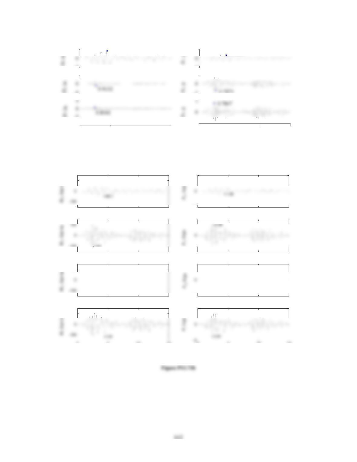
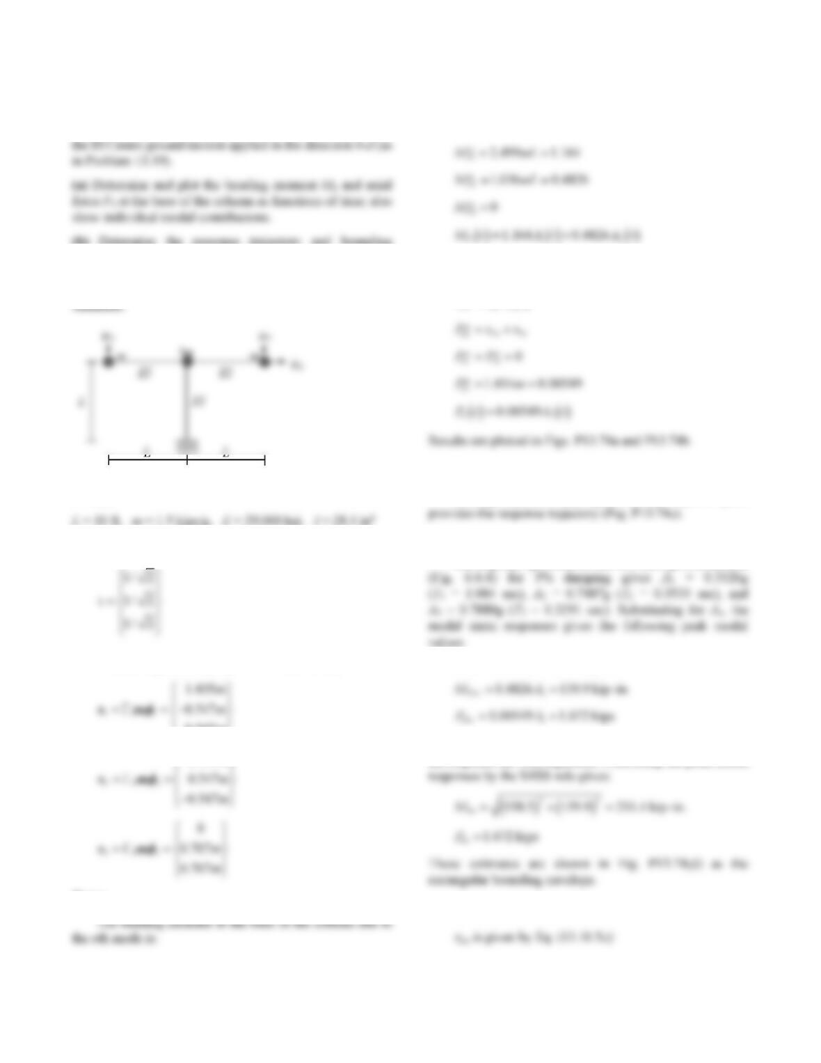
Results are plotted in Fig. P13.73b. Plotting Ma(t) and Pa(t)
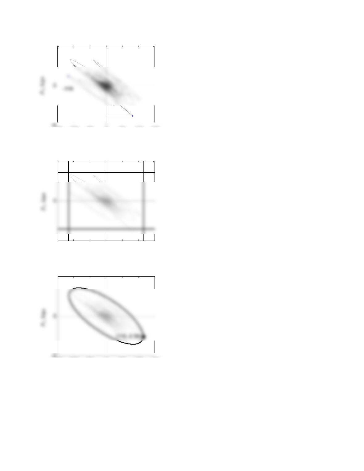
together in the response space provides the response
33
0 0 kip–in.
ao
MA
161
Because the natural frequencies of this system are well
separated, we can combine the peak modal response by the
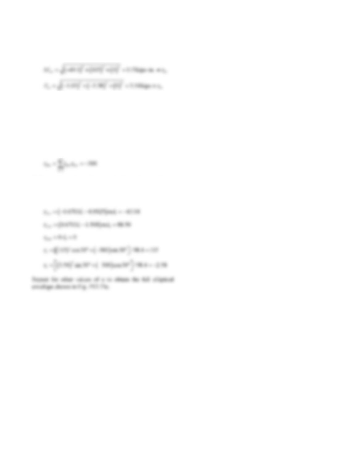
SRSS rule:
These estimates are used to construct the rectangular
envelope shown in Fig. P13.73d.
7. Elliptical bounding envelope.
The coordinates of the elliptical bounding envelope is
given by Eq. (13.10.3), where ao
r and bo
r have already been
determined; abo
ris given by Eq. (13.10.5c):
With ao
r, bo
r, and abo
r known, calculating the coordinates
of the bounding envelope is illustrated for α = 30°:
st
no n n
rrA
P
Figure P13.73a
4.053
-5
5
0.3524
-1
1
-5
5
0.7475
-1
1
-5
0 5 10 15
Time, sec
A
-1
0 5 10 15
Time, sec
0 5 10 15
100
0 5 10 15
-100
104
0 5 10 15
100
0 5 10 15
-5
5
0 5 10 15
-5
5
0 5 10 15
-5
5
0 5 10 15
100
Time, s ec
0 5 10 15
5
Tim e, s ec
D3 in.
163
Figure P13.73c
Figure P13.73d
Figure P13.73e
-150 -100 -50 050 100 150
5
-3.81
M
a
[kip–in]
-150 -100 -50 050 100 150
-5
5
M
a
[kip–in]
-150 -100 -50 050 100 150
5
M
a
[kip–in]
Ma, kip-in.
Ma, kip-in.
Ma, kip-in.
164
Problem 13.74
Consider the system defined in Problem 13.73 subjected to
(b) Determine the response trajectory and bounding
envelopes—rectangular and elliptical—for the two simul-
taneously acting forces Mb and Pb at the base of the column.
1. Data.
2. Influence vector from Problem 9.13:
3. The modal expansion of s (from Problem 13.19):
0.547
2.130
m
m
Part a
st 123
st
bn n
bn
nnn
bn
MMAt
MsLsLsL
The axial force at the base of the column due to the nth mode
is:
st
bn n
bn
PPAt
Part b
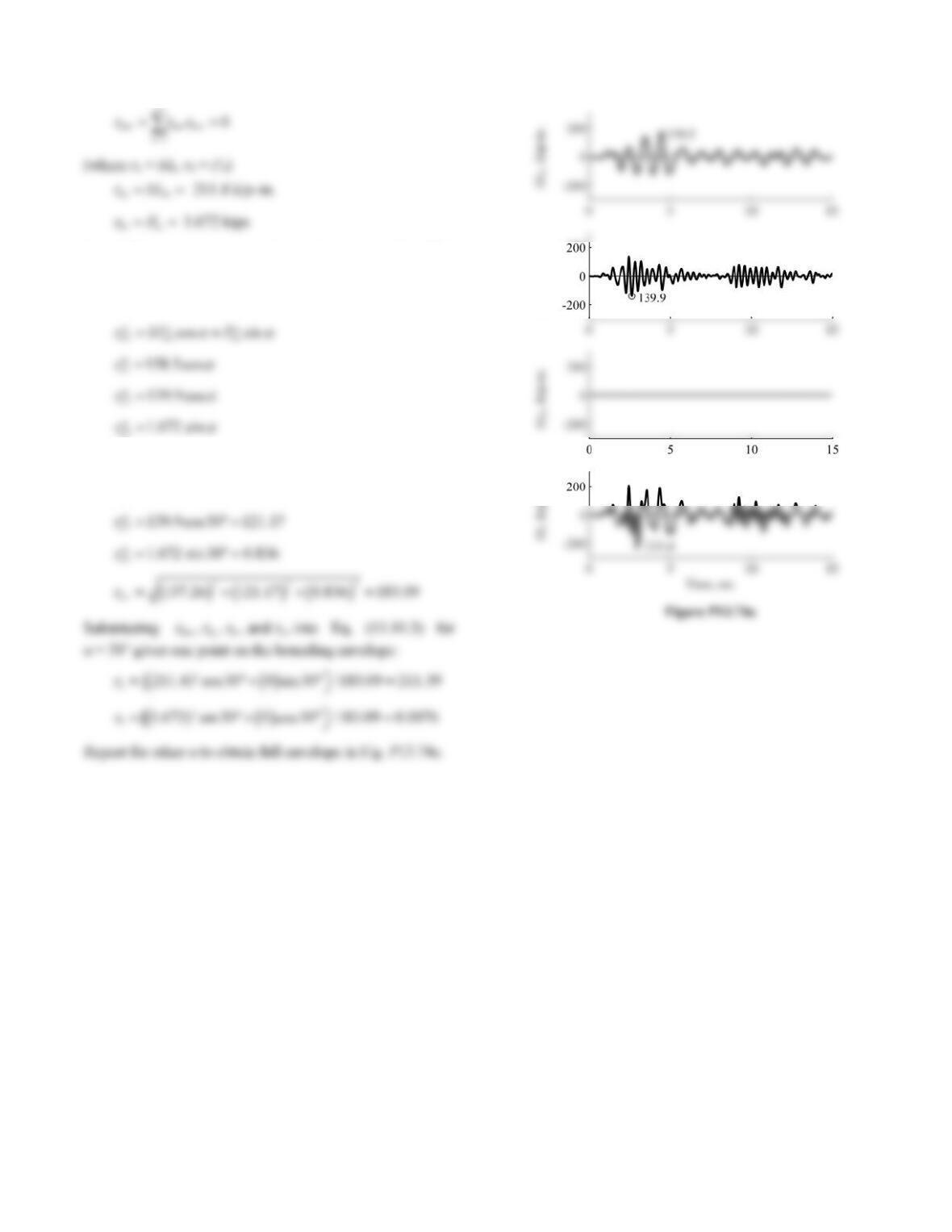
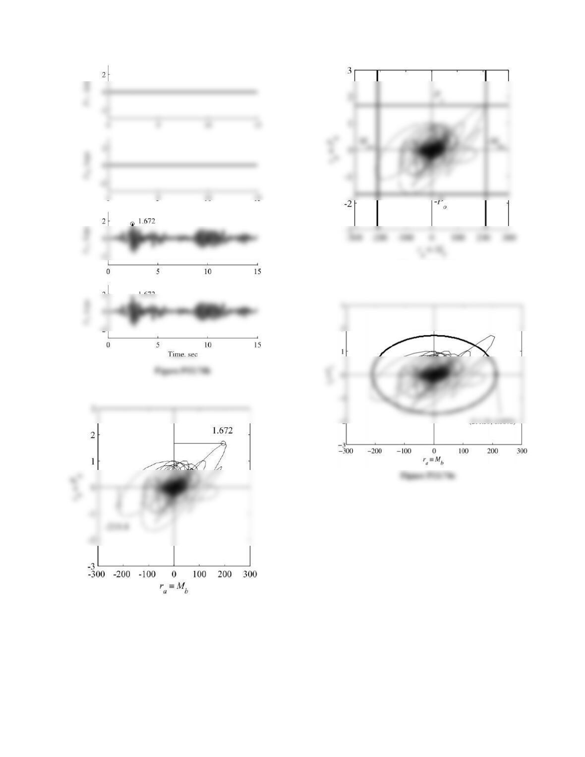
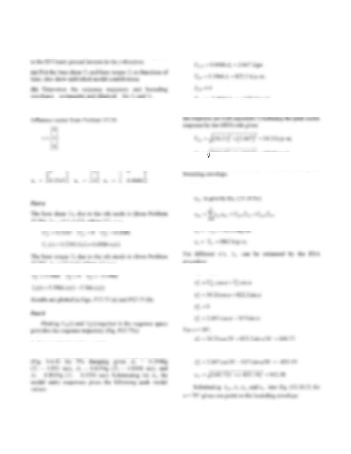
Plotting Mb(t) and Pb(t) together in the response space
4. Rectangular bounding envelope.
The response spectrum for the El Centro ground motion
11
1.164 158.5 kip–in.
bo
MA
The frequencies of the two modes (1 and 2) contributing to
the response are well separated. Combining the peak modal
5. Elliptical bounding envelope.
165
For different α’s, ao
r can be estimated by the RSA
procedure:
st
0
nnn
rrA
For α = 30°,
st
1
158.5cos30 1 37.26
r
166
Figure P13.74c
Figure P13.74d
167
Problem 13.75
The unsymmetric-plan system of Problem 13.26 is subjected
Solution:
The modal expansion of s (from Problem 13.24):
5.3966
0
5.3966
13.26):
st
byn n
byn
VVAt, where 2
byn
Vs
13.26): st ()
bn n
bn
TTAt where st 3n
bn
Ts
1. Rectangular bounding envelope.
The response spectrum for the El Centro ground motion
10 1
20
30 3
0.2245 34.21 kips
0
5.3966 1671 kip–in.
by
by
b
VA
V
TA
The frequencies of the two modes (1 and 3) contributing to
822.2 1671 1862 kip–in.
bo
T
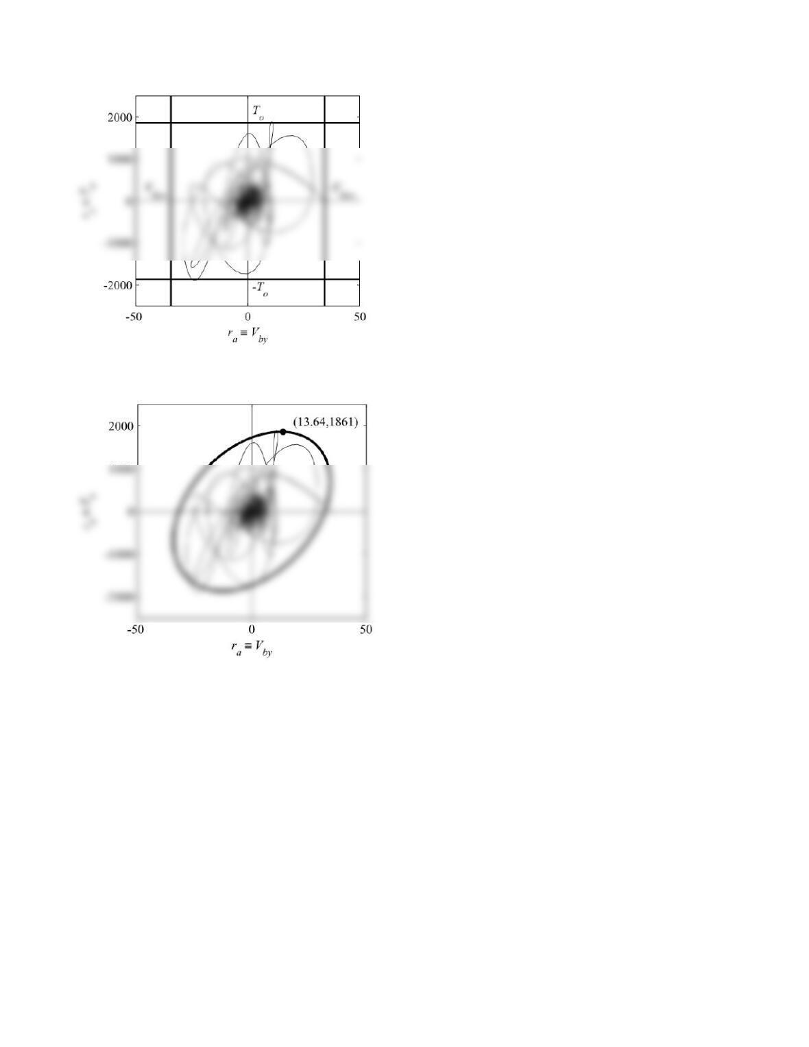
These estimates are shown in Fig. P13.75d as the rectangular
2. Elliptical bounding envelope.
n
st
no n n
rrA
st
2
0
r
168
2
[ 34.31) cos 30 23671 sin 30 / 942.58 13.64
a
r
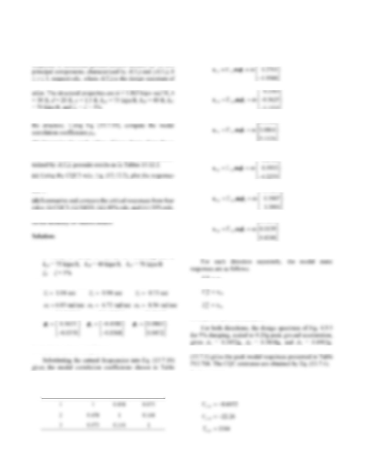
Repeat for other α to obtain full envelope in Fig. P13.75e.
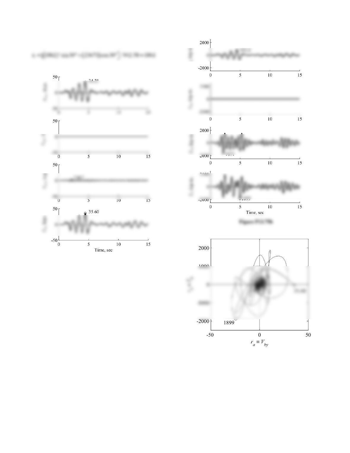
Figure P13.75a
Figure P13.75c
Tb1, kip-in. Tb2, kip-in.
169
Figure P13.75d
Figure P13.76e
170
Problem 13.76
The one-story, two-way unsymmetric system of Fig. 9.5.1 is
subjected to horizontal ground motion defined by its two
Fig. 6.9.5 (ζ = 5%) scaled to 0.20g peak ground acceler-
(a) Determine the natural periods and modes of vibration of
(b) Determine the peak values of base shears along the x–
and y-axes, Vbx and Vby, respectively, and base torque Tbz,
due to individual components of ground motion charac-
incident angle relation for four values of γ: 0.50, 0.67, 0.85,
and 1.
Present results as in Tables 13.12.4 and 13.12.5. Comment
1. Data.
b = 30 ft, d = 20 ft, e = 1.5 ft, m = 1.863 kip–sec2/ft
2. Natural vibration properties.
0.2622 0.4249 0.5362
3. Modal correlation coefficients.
P13.76a.
Table P13.76a: Modal Correlation Coefficients
in
Mode, i n = 1 n = 2 n = 3
4. Modal expansion of s.
For the x-direction,
0.1280
3.1535
For the y-direction,
0.2761
0.3625
0.0864
5. Modal static responses.
x
nn
Vs
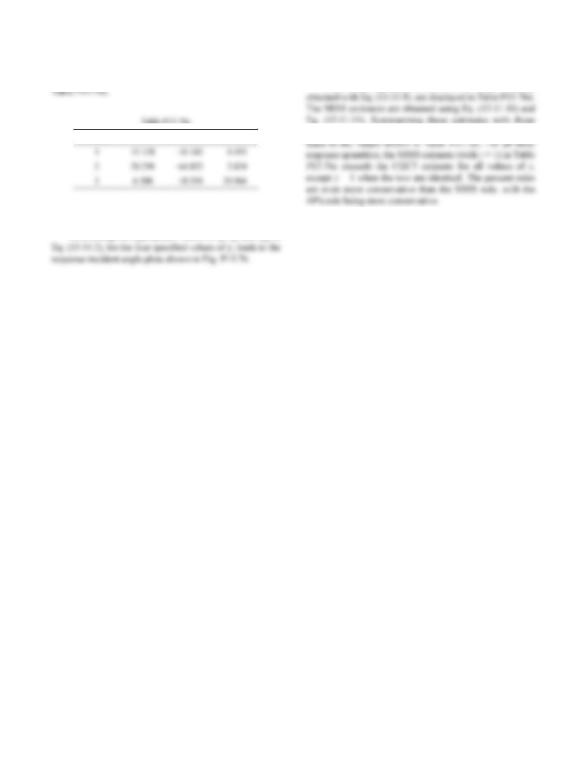
6. Response spectrum analysis.
Substituting the modal static responses and An in Eq.
7. Cross terms.
11
NN
x
yinixny
in
rrr
171
For base shear in the x-direction Vx, the individual terms
in the double summation of Eq. (13.11.5) are presented in
Table P13.76c
Mode, i n = 1 n = 2 n = 3
8. Response-incident angle relations.
Substituting the appropriate values of ݎ
9. Critical response estimates.
The critical response estimates from the CQC3 method,
from the percent rules, as obtained from Eq. (13.11.13),
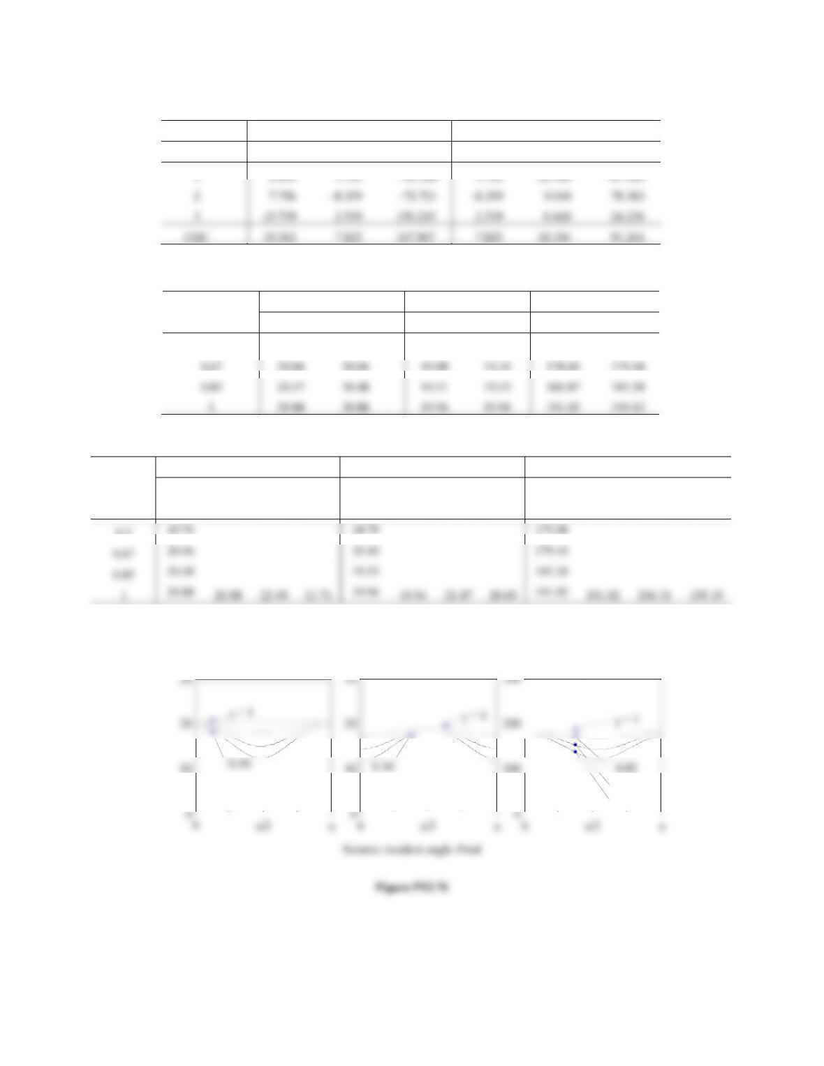
172
Table P13.76b
Excitation x-direction y-direction
Mode Vx (kips) V
y (kips) T
z (kip–ft) V
x (kips) V
y (kips) T
z (kip–ft)
Table P13.76d
Intensity Ratio γ
Vx (kips) Vy (kips) Tz (kip–ft)
SRSS CQC3 SRSS CQC3 SRSS CQC3
0.5 19.75 19.76 18.76 18.79 173.90 175.08
Table P13.76e
γ
Vx (kips) Vy (kips) Tz (kip–ft)
CQC3 SRSS
40% 30%
CQC3 SRSS
40% 30%
CQC3 SRSS
40% 30%
Rule Rule Rule Rule Rule Rule
0.5 19.76
(a) V
bx
, kips
(b) V
by
, kips
(c) T
bz
, kip-in.
0.67
0.50