Now atm
p
pp
12
== and ≈
10V. This gives (for
α
=
21.0)
For screwed connections,
ent
K
1.0=, check
K
2.0=, elb
K
0.6
4
=, tee
K
0.90=, gate
K
0.11=, globe
K
5.7=
These numerical values give
For 10 C water, the Reynolds number is
We next tabulate the required head p
h for each flowrate Q.
Q (m3/s) Ref
Required
Head, hp (m)
Pump head, hp
(m)
0 0 0 40 60
0.010 9.72 × 1040.0206 43.5 64.4
Plotting these values on the same graph as the pump head-flow curve gives p
h59
m
≈ and
=3
0.023m /sQ
Problem 12.26
A centrifugal pump having an impeller diameter of
1
m is to be constructed so that it will
supply a head rise of 200m at a flowrate of 3
4.1m /s of water when operating at a speed of
1
200 rpm. To study the characteristics of this pump, a
1
/5 scale, geometrically similar model
operated at the same speed is to be tested in the laboratory. Determine the required model
discharge and head rise. Assume that both model and prototype operate with the same
efficiency (and therefore the same flow coefficient).
Solution 12.26
For similarity, the model pump must operate at the same flow coefficient so that
and with mp
ω
ω
=, mp
D
D/1/5=, and p
Q3
4.1m /s=, then
()
m
Q
333
1m m
1 4.1 0.0328
5s s
==
From Eq. (12.33)
ω
D
Problem 12.27
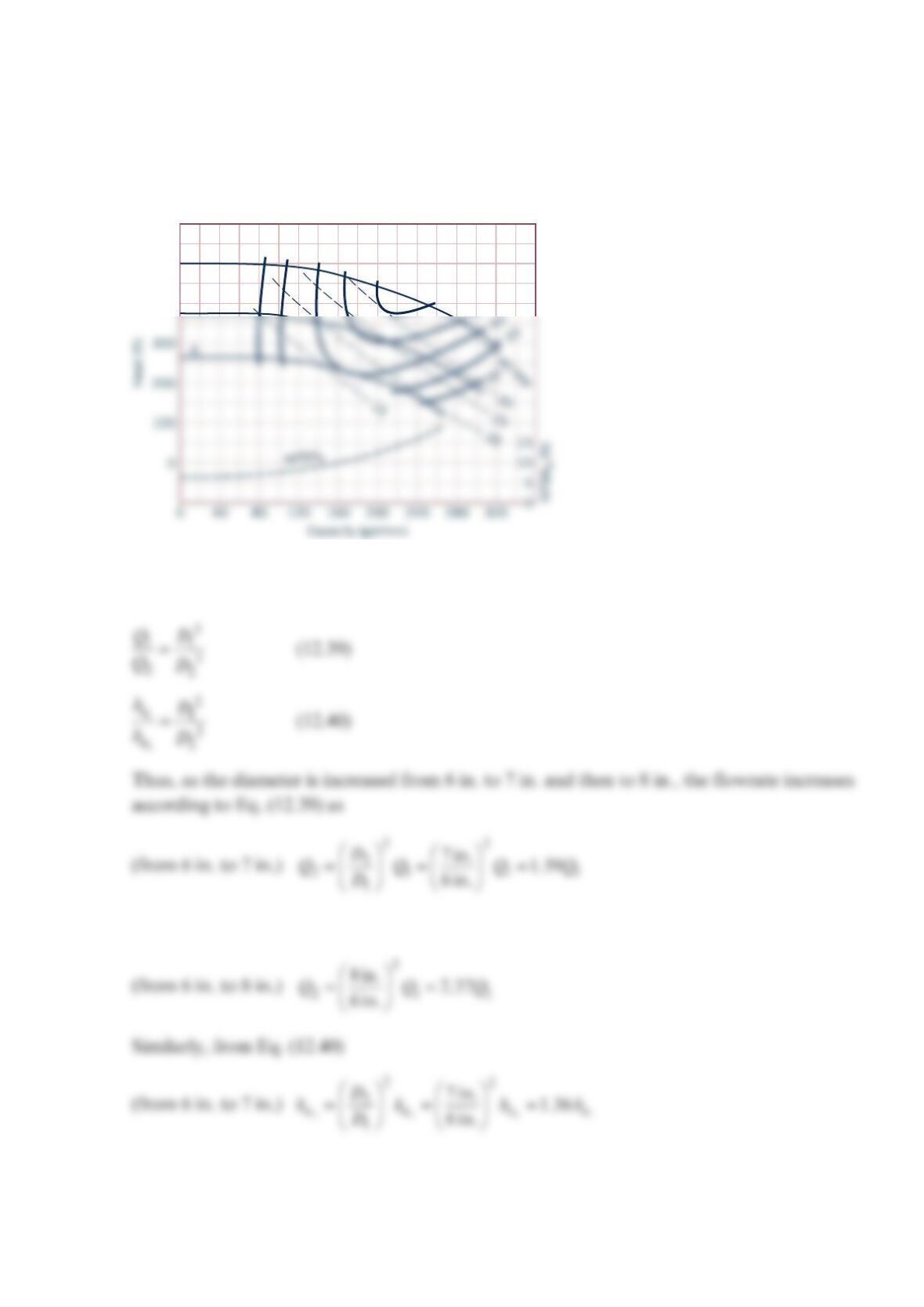
Do the head–flowrate data shown in Fig. 12.12 appear to follow the similarity laws as
expressed by Eqs. (12.39) and (12.40)? Explain.
Solution 12.27
The data in the Fig.12.12 show the effect of changing impeller diameter on head-flowrate
characteristics. The similarity laws expressed by Eqs. (12.39) and (12.40) are
and
8 in. dia
7
50%
55
60
63
65
65
400
500
and
Thus, for any gives point, such as (A) where =120 gpmQ and a
h
250 ft= (see Fig. 12.12) for
the 6-in. diameter impeller, the corresponding predicted point would be at (B) Where
()( )
==
21.59 120 gpm 191gpmQ
()( )
a
h
21.36 250 ft 340 ft==
Similarly, for the
8
-in.
diameter impeller, the predicted point, point (C), would be at
Points (B) and (C) fall near the corresponding curves in Fig. 12.12 thereby demonstrating
that they do appear to follow the similarity laws. Yes.
Problem 12.28
A centrifugal fan operating in a duct has the dimensionless parameters
ω
=
Q3
Q
CD and
ρω
Δ
=
H22
p
CD,
where Q
C is a flow coefficient, H
C is a head coefficient,
Q
is the volume flowrate,
ω
is the
fan speed,
D
is the fan diameter,
ρ
is the fluid density, and
Δ
p
is the fan pressure rise. The
figure below shows this fan’s performance curve in dimensional form for a fan speed of
ω
=
15 1500 rpm. Find the fan operating points (
Q
and
Δ
p
) for
ω
=
30 3000 rp
m
and
corresponding to points 1, 3, and 5 at
ω
=
15 1500 rp
m
. Assume similarity between
1
500 rpm
and
3
000 rpm.
Solution 12.28
The two dimensionless groups,
φ
=
Q()C and
ψ
=
H()C give
15
15
Then
012
2
3
3
4
45
0
11
2
3
4
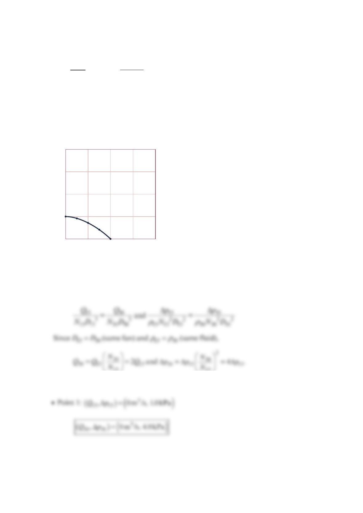
Volume flow rate, Q (m3/s)
Fan pressure rise, Δ
p
(kPa)
Δp = 1 – 0.25 Q2
N15 = 1500 rpm

•
Point 3:
()
()
Δ= 3
15 15
, 1.0 m /s, 0.75 kPaQp
•
Point 5:
()
()
Δ= 3
15 15
,2.0m/s, 0kPaQp
Problem 12.29
A centrifugal pump has the performance characteristics of the pump with the 6-in.-diameter
impeller described in Fig. 12.12. Note that the pump in this figure is operating at
3
500 rpm.
What is the expected head gained if the speed of this pump is reduced to
2
800 rpm while
operating at peak efficiency?
Solution 12.29
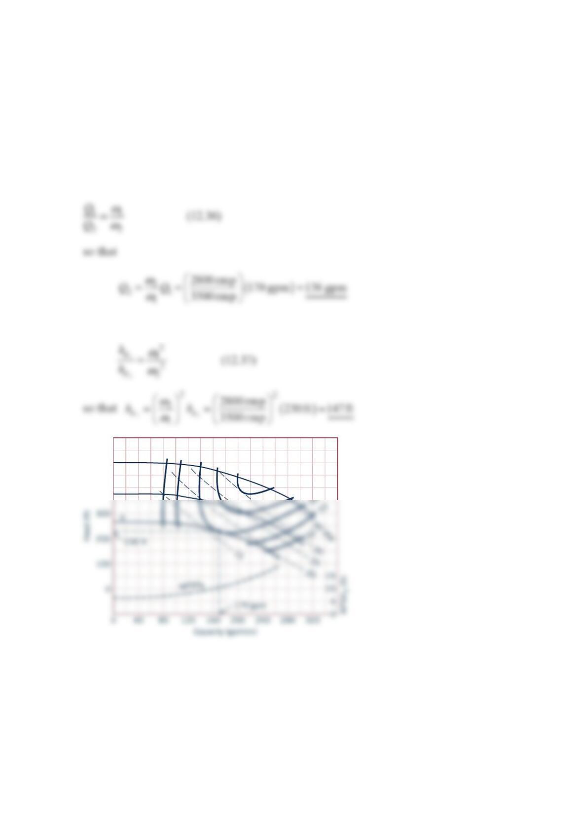
From Fig. 12.12, for the 6-in. diameter impeller operating at
3
500 rpm, =170 gpmQ, and
=
a230 fth when operating at peak efficiency (see the figure below). Thus, if the pump is
still operated at peak efficiency with the speed reduced to
2
800 rpm then from Eq. (12.36)
From Eq. (12.37)
8 in. dia
7
50%
55
60
63
65
63
65
400
500
Problem 12.30
A prototype fan has a 20-ft diameter, an inlet pressure of
1
4.40 psia, an inlet temperature
of 70 F, and a speed of
9
0rpm.
A 1
10-scale model of the fan has the same inlet pressure and
temperature, an inlet power of
1
.24 hp, a flowrate of 3
220 ft /min, and a speed of
1
800 rpm.
Find the corresponding input power and flowrate of the prototype fan. Neglect Reynolds
number effects.
Solution 12.30
The scaling law for power is
Problem 12.31
Use the data given in Problem 12.18 and plot the dimensionless coefficients H
C
, P
C
,
η
versus
Q
C
for this pump. Calculate a meaningful value of specific speed, discuss its
usefulness, and compare the result with data of Fig. 12.18.
Solution 12.31
From Problem 12.18, the following data were obtained:
Q (gpm) 20 40 60 80 100 120 140
Based on the data above:
Q (gpm) 20 40 60 80 100 120 140
CQ5.76 ×
10−4
1.15 ×
10−3
1.73 ×
10−3
2.30 ×
10−3
2.88 ×
10−3
3.46 ×
10−3
4.03 ×
10−3
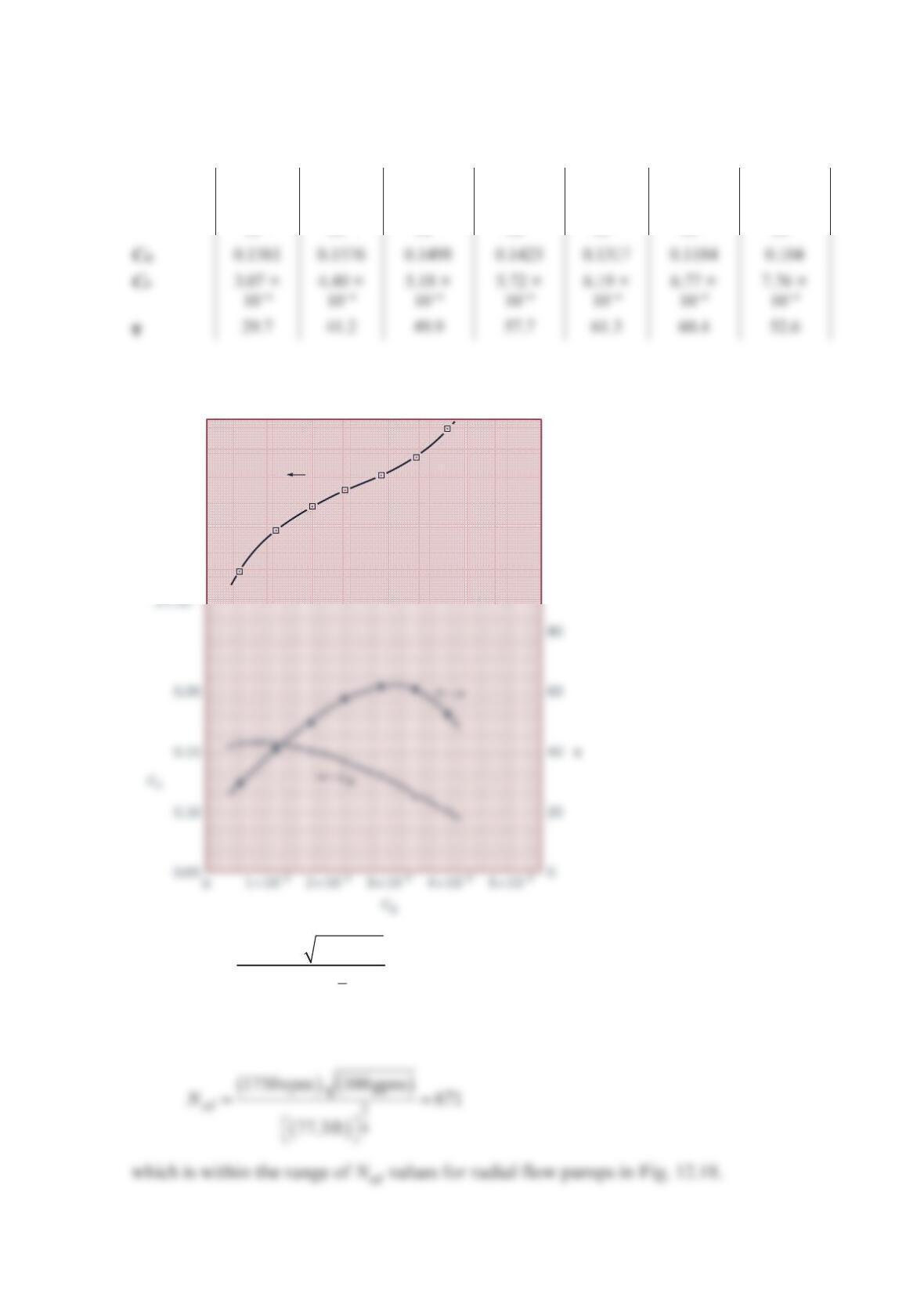
The plot of H
C
, P
C
,
η
versus
Q
C
is shown below.
()()
()
sd
Q
N
h
3
4
a
rpm gpm
ft
ω
=
So for max
Q100 gpm at 61.3%
η
==
–4
4
×10
–4
6
×10
–4
8
×10
–4
C
P
C
P
Problem 12.32
In a certain application, a pump is required to deliver 5000 gpm against a
3
00-ft head when
operating at 1200 rpm. What type of pump would you recommend?
Solution 12.32
For =5000 gpm,Q a
h
300 ft,= and
ω
=1200rpm, the specific speed is
Problem 12.33
A centrifugal pump operates at
3
00 rpm to deliver 20 C lubricating oil. A 1–
5size,
geometrically similar pump delivering 15 C water is used to model the larger pump. How
fast should the smaller pump run? Discuss the accuracy of the result.
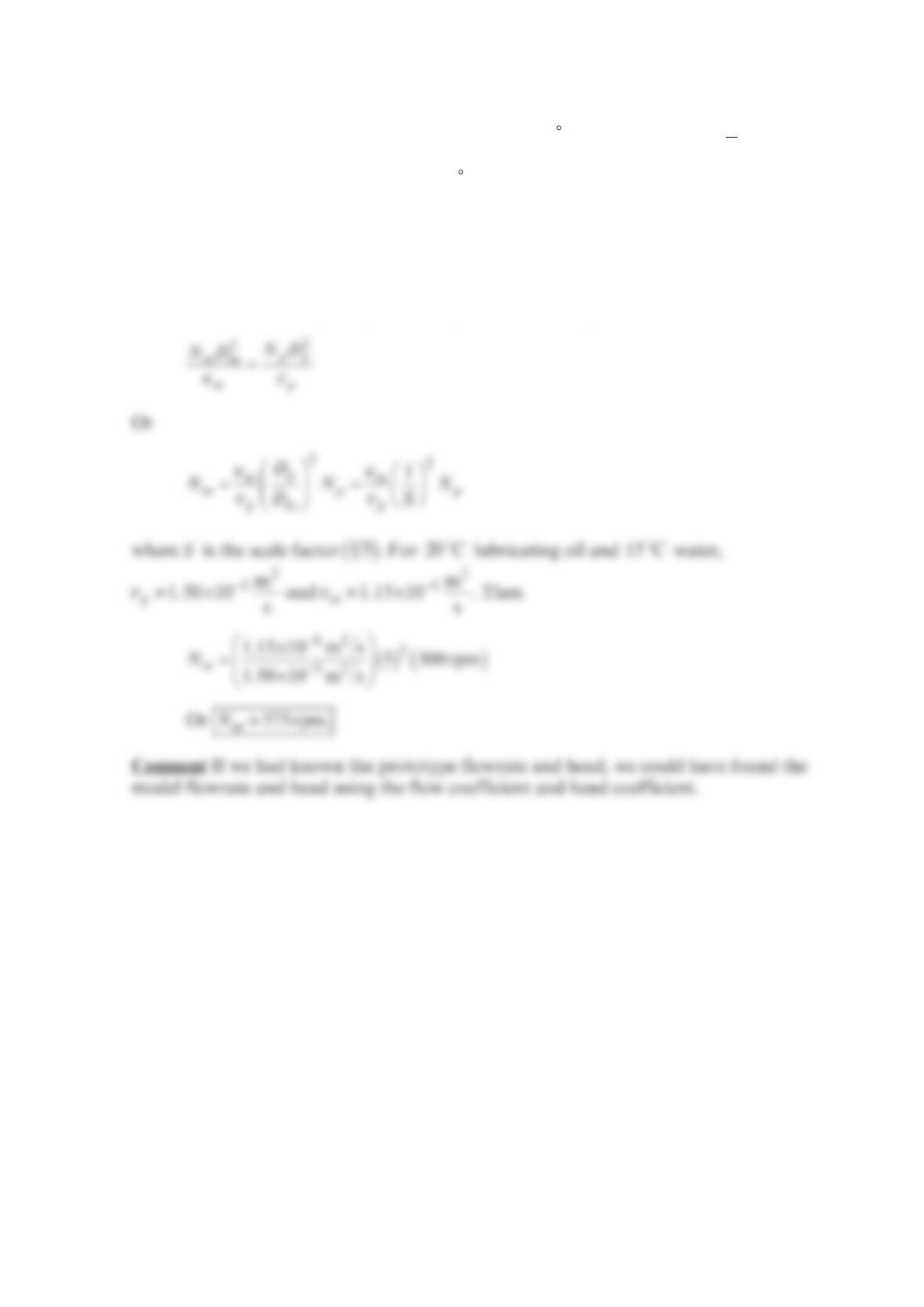
Solution 12.33
The relevant dimensionless groups for a centrifugal pump are the flow coefficient, the head
coefficient and the Reynolds number. Because the pump is handling a viscous fluid, Re
should be considered. Equality of the Reynolds numbers gives
Problem 12.34
A certain axial-flow pump has a specific speed of s
N5.0.= If the pump is expected to deliver
3
000 gpm when operating against a
1
5-ft head, at what speed
()
rpm should the pump be
run? Draw a sketch of the pump impeller (front and side views).
Solution 12.34
Since
()
()
()
()
s
Q
N
gh
3
3
24
a
rad s ft s
ft s ft
ω
=
Problem 12.35
A certain pump is known to have a capacity of 3
3m /s when operating at a speed of
60 rad/s against a head of 20 m. Based on the Hydraulic Institute/Worthington Specific
Speed Chart, would you recommend a radial-flow, mixed-flow, or axial-flow pump? Draw
a sketch of the pump impeller (front and side views).
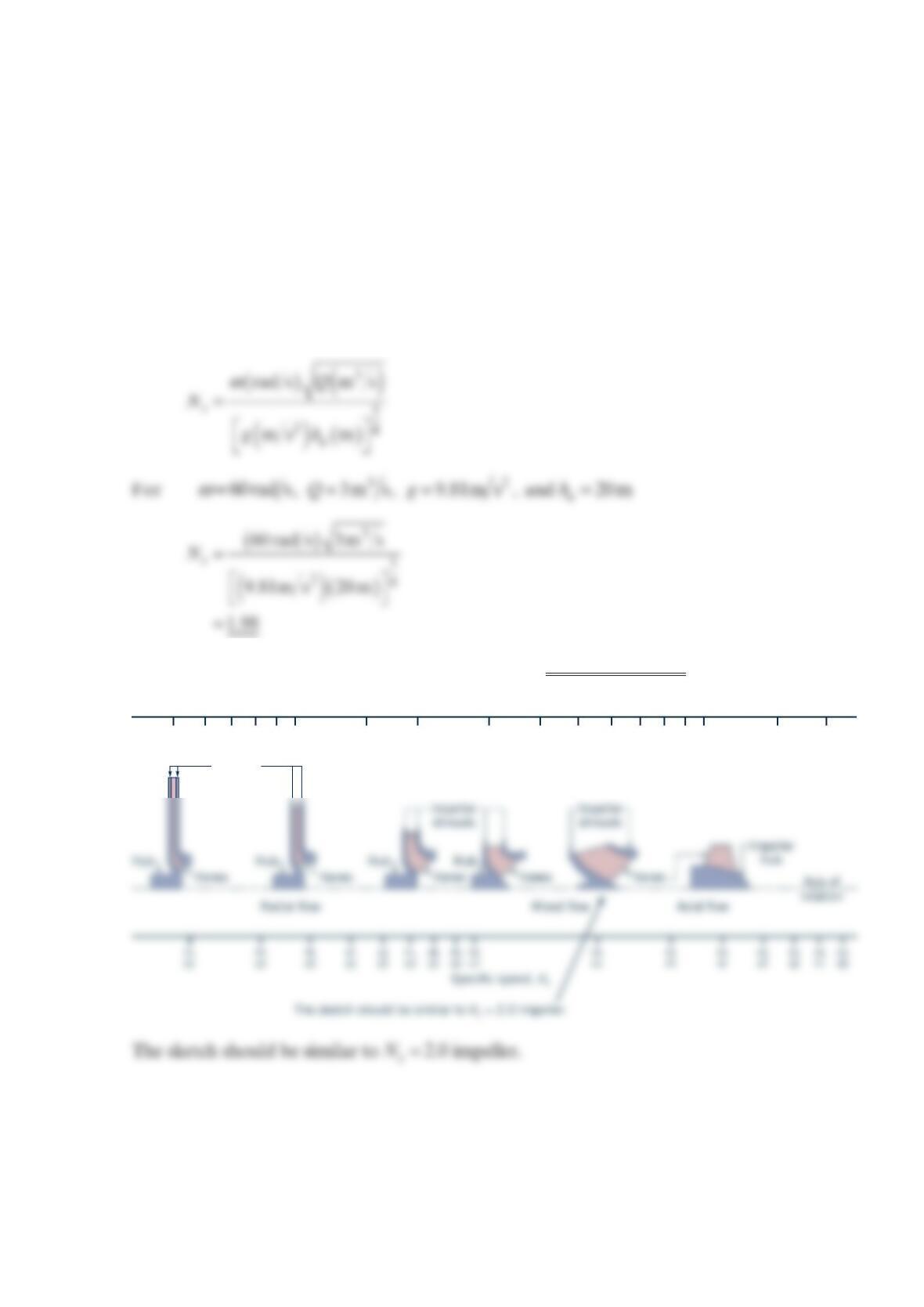
Solution 12.35
Since
From the figure below with s
N1.9
8
=, the pump is a mixed-flow pump.
500
600
700
800
900
1000
1500
2000
3000
4000
5000
6000
7000
8000
9000
10000
15000
20000
Specific speed, N
sd
Impeller
shrouds
Problem 12.36
The system resistance for a pipeline is given by sys
p
Q2
2.0 ,
Δ
= where Δsys
p is the pressure
rise required of a pump to deliver the flowrate
Q
through the piping system. A pump has
the pressure-rise–flow characteristic given by p
p
Q2
30.0 3.0 .
Δ
=− In both curves,
Δ
p
is in
k
Pa and
Q
is in 3
m
/s. Find the pump input power if this pump is placed in this piping
system and the pump overall efficiency is
9
0%.
Solution 12.36
The pump-system matching condition is psys
hQ h Q() (
)
= so
Problem 12.37
The axial-flow pump shown in the figure below is designed to move 5000 gal/min of water
over a head rise of 5ft. Estimate the motor power requirement and the
θ
22
UV needed to
achieve this flowrate on a continuous basis. Comment on any cautions associated with
where the pump is placed vertically in the pipe.
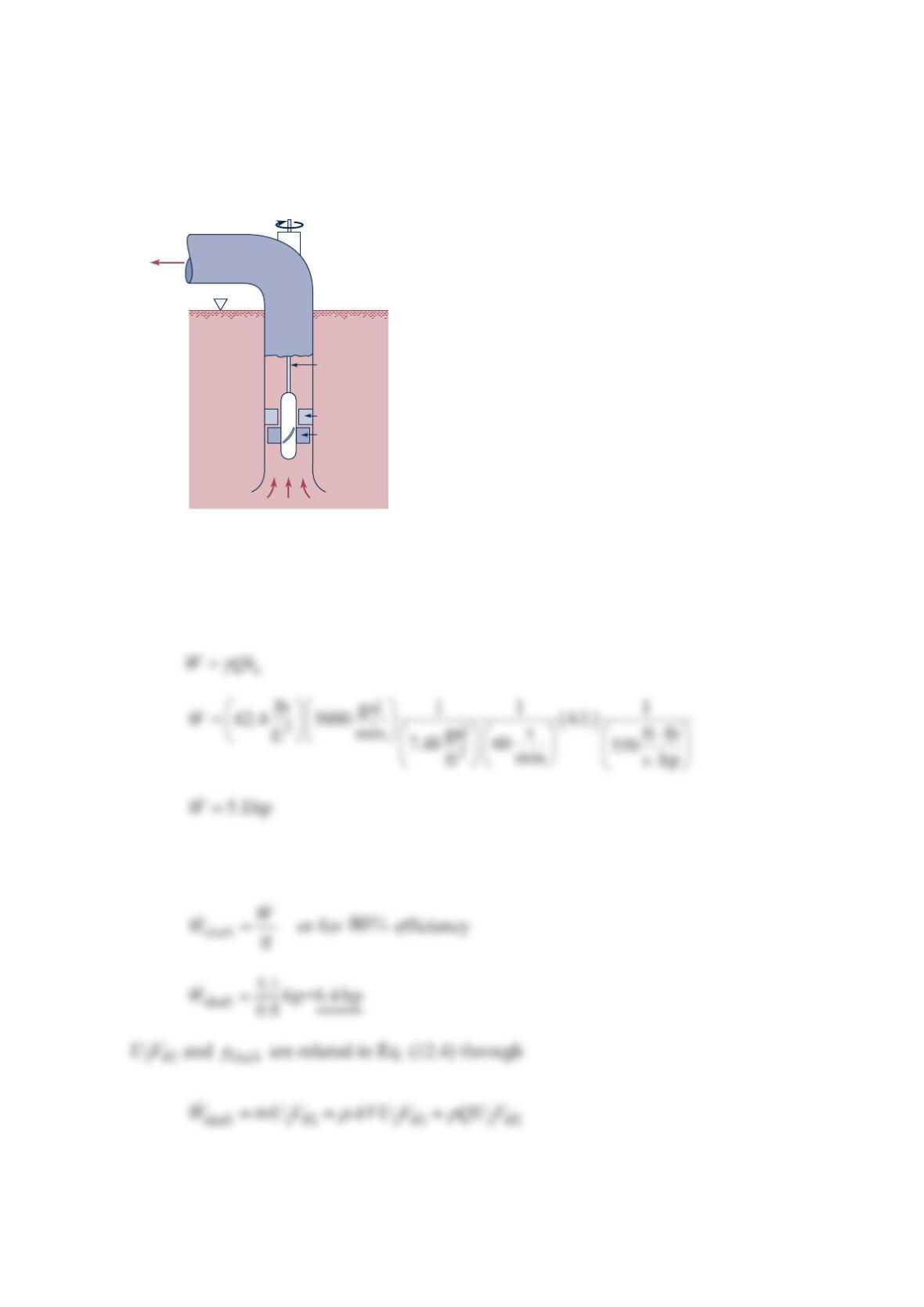
Solution 12.37
From Eq. (12.21), we get the power equivalent to the head rise and flowrate involved. This
is the minimum power required to achieve the performance specified.
To estimate the shaft or motor power requirement, we need to assume the efficiency of the
conversion of shaft or motor power into the pump performance specified.
Inlet
Discharge
Rotor blades
Fixed stator blades
Drive shaft
Shaft to motor
So
The main caution in placing the pump vertically in the intake pipe is to do so in a way to
avoid cavitation in the pump. The collapse of cavitation bubbles in the pump can erode
pump blades and other wetted surfaces. Applying the energy equation, Eq. (5.84), between
the free surface (1) and the pump entrance (2), we get
Problem 12.38
A propeller-driven airplane is traveling with a velocity
()
=
1200 mph 294 ft/s .V The
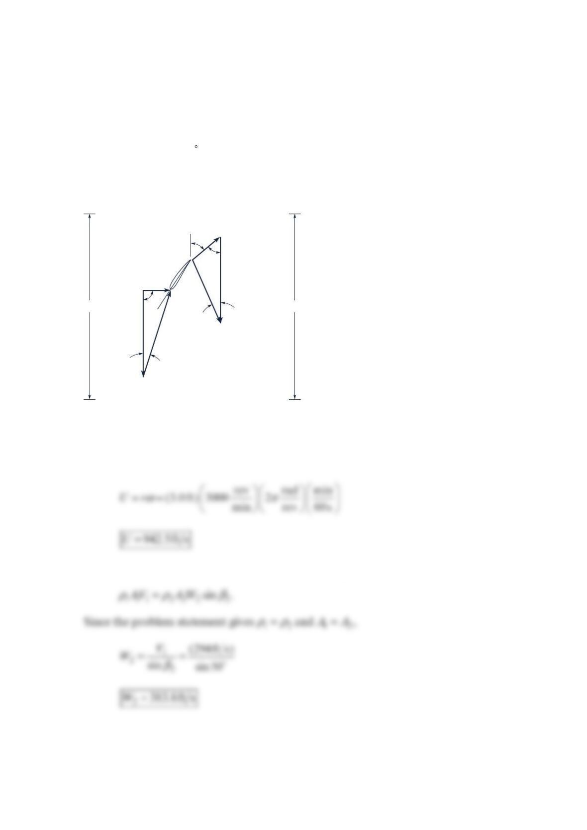
propeller diameter is 10 ft and it rotates at 3000 rpm. The figure below shows a propeller
cross-sectional profile and the velocity diagrams for a short section of the propeller at a
radius of 3.0 ft. The outlet relative velocity 2
W
is assumed tangent to the propeller at the
outlet, so
ββ
′==
12
50 . The air density is constant as it flows over the propeller. Assume
that the flow area for the mass flowrate interacting with this short section of the propeller is
the same upstream and downstream (inlet and outlet) from the propeller (i.e., =
1
2
A
A).
Produce the velocity diagram downstream from the propeller by finding ,U 2,
W
2,
V
and
α
2.
Solution 12.38
The propeller velocity
U
is
Conservation of mass for a control volume enclosing the short section of the propeller gives
A
The velocity 2
V is found from the law of cosines,
U
U
W
2
W
1
V
2
V
1
A
2
1
′
β
2
β
2
β
1
α
2
α
A
1
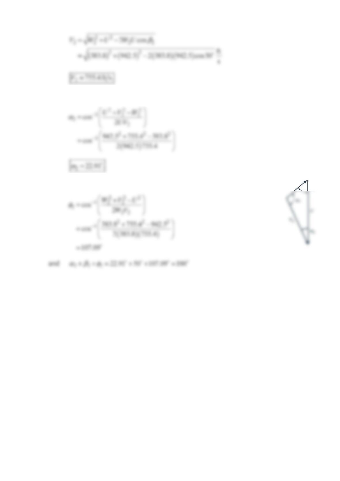
The angle
α
2 is found from the law of cosines,
As a check, the law of cosines gives
W
2
2
β