20
Problem 12.15
and combined.
t
r
t
Solution:
t, sec
0.15
100
1. Determine natural frequencies and modes and
M
n.
2. Set up modal equations.
M
K
P
t
t
ttt
3. Solve modal equations.
t
where p
t
() is a step force po with rise time
t
r
is
(c)
In Eq. (c), replacing po by 100 kips, and k by
qt
t
2
0 576 10
015
15 0015
015
() .()
.
..sec
.sec
H
GI
K
J
S
|
|
T
t
015
.sec
T
(e)
4. Combine modal responses.
The total displacements are
In Eq. (f),
and q
t
t
. sec and by
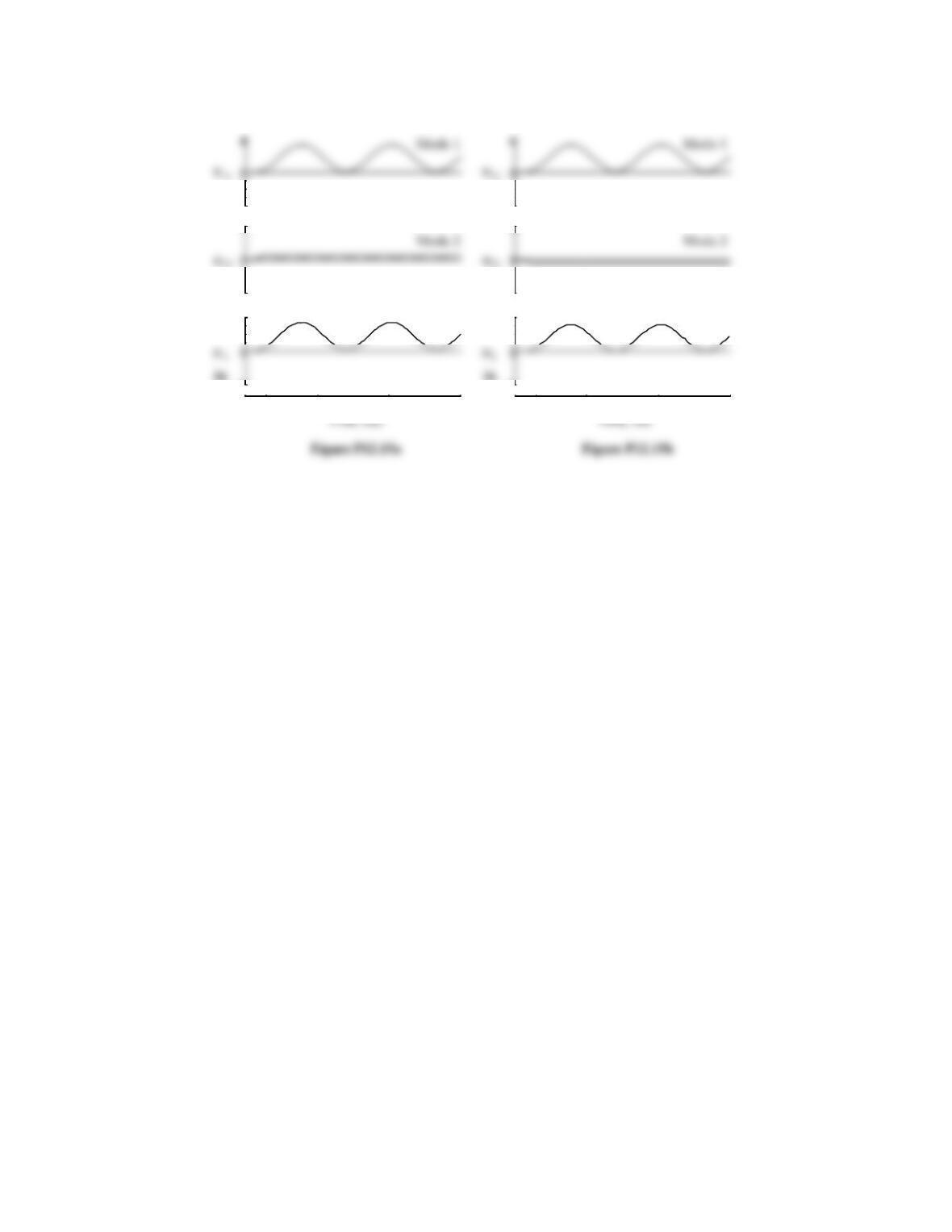
The modal responses and total response are plotted in
Figs. P12.15a–b.
21
-4
-1
1
-4
-1
1
-4
4
-4
4
Total Total
0 0.5 1 1.5
0.15 0 0.5 1 1.5 0.15
22
Problem 12.16
Determine the displacement response of the system of
Problem 12.13 to force p(t), which is shown in Fig. P12.16
and applied at the right mass. Plot as functions of time the
displacements uj(t) due to each vibration mode separately
and combined.
Solution:
t
p (t) = p(t)
2
t, sec
0.30
p, kips
M
M
K
P
t
t
t
t
t
t
t
t
t
11 2
t
() () () 0
T
d
Pt t p t tt
p
(b)
3. Solve modal equations.
t
t
t
t
t
t, sec
p
td
o
The solution of Eq. (c) is
(d)
For mode 1,
Substituting in Eq. (d) for
t
t
d
gives
Substituting in Eq. (d) for
t
t
d
gives
23
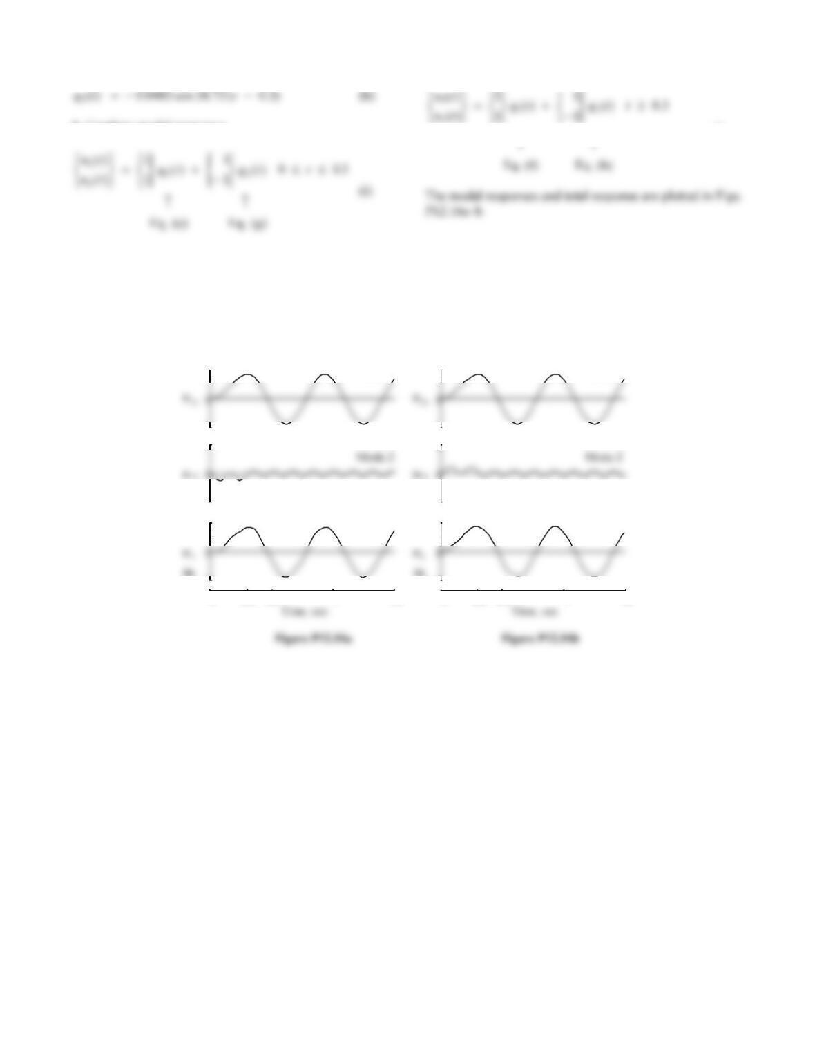
4. Combine modal responses.
(j)
-4
4
-1
1
-4
4
-1
1
-4
4
-4
4
Mode 1 Mode 1
Total Total
0 0.5 1 1.5
0.3 0 0.5 1 1.5 0.3
24
Problem 12.17
Solution:
From Example 12.6,
ut
ut
00214 00286
()
..
()
R
L
2. Write force-displacement relations.
V
EI
LL
u
a
b
e
a
b
|
|
|
|
M
M
P
P
|
|
|
|
12 6 6
k
(d)
3. Determine forces in element 1.
V
qq
d
R
U
R
U
R
U
S
|
|
V
|
|
12
12
0
0
666 03 7019
.
4. Determine forces in element 2.
12
12
0.3274 1.5274
251.3 6650.7
Vu q q
qq
411
4.80 6.88
12.6.
25
Problem 12.18
diagrams due to each mode separately and combined.
1. Determine natural frequencies and modes.
From Problem 12.13,
2. Determine equivalent static forces for each mode.
t
t
ft qt qt
21
11
1
1
28 8
() () . () .
.()
S
TU
V
WL
N
MO
Q
PR
S
TU
V
WR
S
TU
V
W
(a)
t
t
(b)
3. Combine modal forces.
t
t
t
4. Determine internal forces.
By statics, the reactions are
Static analysis gives the bending moment
M
t
M
t
af
() ()
0
Static analysis gives the shears:
12
112
21
() () () ()
33
33
ab
cA
Vt Vt ft ft
5. Determine modal coordinates at
t
01. sec.
From Problem 12.14,
At
t
01. sec
6. Determine internal forces at
t
01. sec.
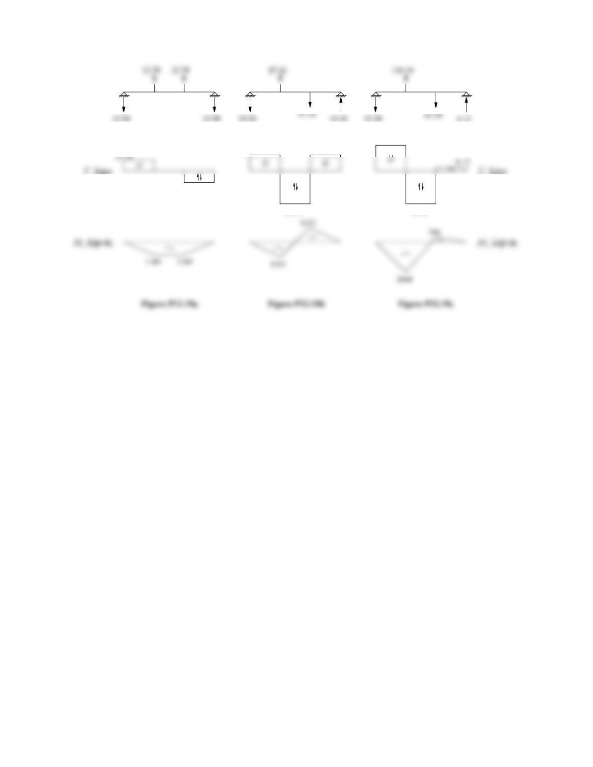
Substituting Eq. (h) in Eq. (a) and Eq. (b) gives
26
f
(t), kips
S
22.98
52.08
f (t), kips
S
29.10 29.10
58.16 58.16
Problem 12.19
and ω = 25 rad/sec. Neglecting damping, determine the
forced (or steady-state) response of the system. In
particular, determine:
(a) the displacements and accelerations of the two masses
as functions of time; and
(b) the amplitudes of displacements and accelerations.
Solution:
u (t)
1u (t)
2
1. Determine natural frequencies and modes.
See Problem 12.13.
2. Set up modal equations.
3. Solve modal equations.
4. Determine displacements and accelerations.
R
R
t
12
0133 25
() ()
.sin
5. Determine amplitudes of displacements and
accelerations.
TU
WR
TU
W
28
Problem 12.20
For the system and excitation of Problem 12.19, determine
the amplitude of the forced (or steady-state) bending
moment at the location of each mass by using equivalent
static forces.
Solution:
1. Determine equivalent static forces.
From Problem 12.18,
2. Determine modal coordinate amplitudes.
From Problem 12.19,
t
t
t
t
To determine the response amplitude we specialize Eq. (b)
when sin 25 1
t
; thus
Substituting qno for q
t
n() in Eq. (a) gives
o
2
3. Determine bending moments.
From Eq. (e) of Problem 12.18,
t
t
t
29
Solve Problem 12.19 assuming modal damping ratios of
10% for the system.
See Problem 12.13.
3. Solve modal equations.
where
2
1( )
n
For the first mode,
Substituting these numerical values in Eqs. (c)–(e) gives
10 328 25 0 031 25( ) . sin . cos
For the second mode:
4. Determine displacements.
() ()
5. Determine displacement amplitudes.
6. Determine acceleration amplitudes.
30
Problem 12.22
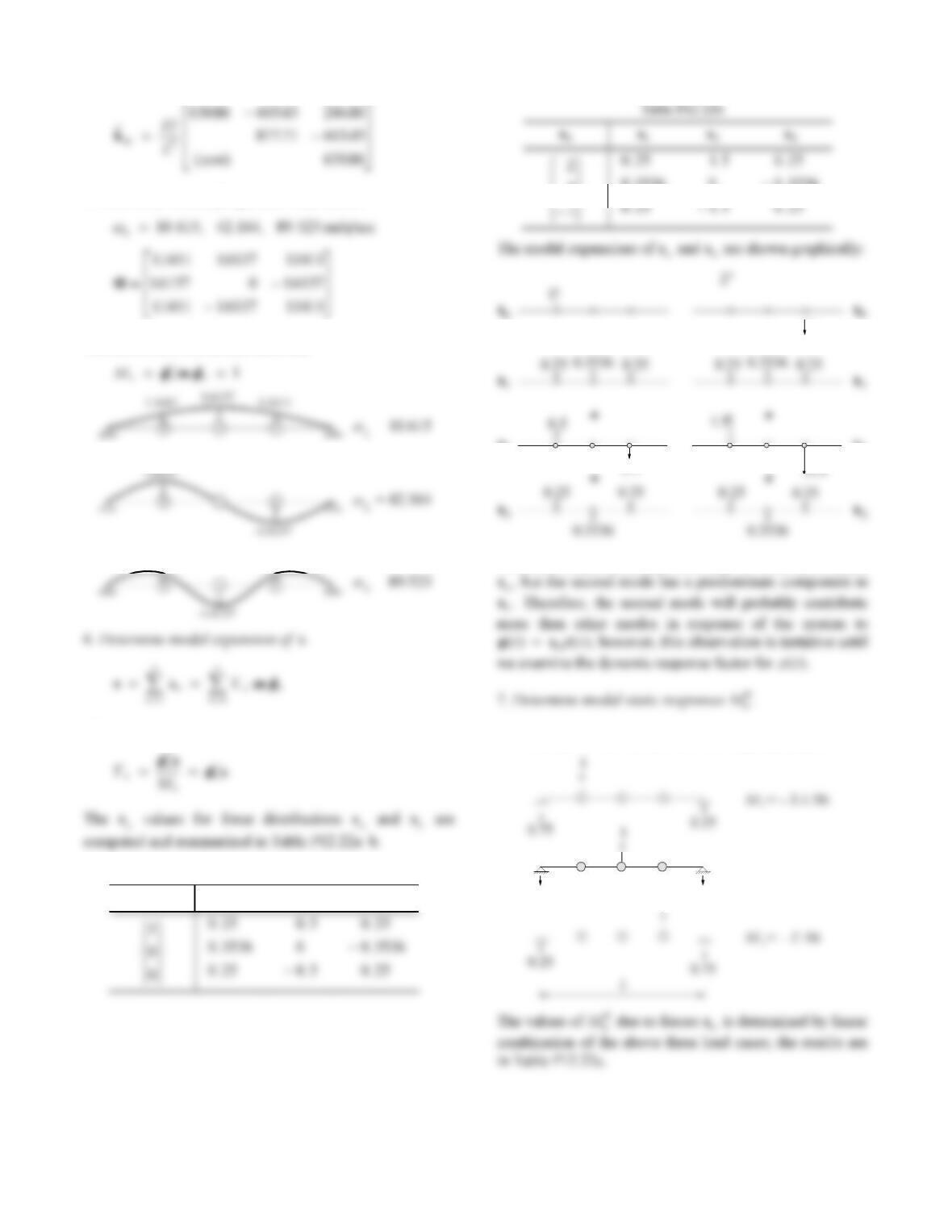
Figure P12.22 shows a massless simply supported beam
with three lumped masses and the following properties:
L = 150 in., m = 0.192 kip–sec2/in., E = 30,000 ksi, and
I = 100 in4. We are interested in studying the dynamic
response of the beam to two sets of applied forces: p(t) =
sp(t), sT
a = 1 0 0, and sT
b = 2 0 −1.
(a) Determine the modal expansion of the vectors sa and sb
that define the spatial distribution of forces. Show these
contribution factors and the error eJ are influenced by the
spatial distribution of forces.
half-cycle sine pulse:
L
of the system. Figure 12.11.3 gives the shock spectrum for
a half-cycle sine pulse with numerical ordinates Rd =1.73,
1.14, and 1.06 for T1/td = 1, T2/td = 0.252, and T3/td =
0.119, respectively. It should be convenient to organize
factors Rdn, and the force distributions sa and sb.
(f) Can you determine the peak value of the total (con–
Figure P12.22
Solution:
1. Define DOFs.
2. Determine mass matrix in terms of ut.
3. Determine stiffness matrix.
L
O
LL LL
22
72 036 0
4. Determine lateral stiffness matrix.
31
5. Determine natural frequencies and modes.
The modes are normalized such that
t
t
t
1.1411 1.1411
where
Table P12.22a
sa s1 s2 s3
0
S
|
V
|
0 3536
.
0
0 3536
.
=
=
0.5
s2
s2
1
All three modes contribute similarly to force distribution
First determine
M
1 for the following load cases:
1
0.5 0.5
M = – L /8
1
Mode, n Mn1
1 – 0.1067L – 0.1067L
Next we determine M1
st :
1
2
16 0 1875 5
16 0 3125 ..
8. Determine modal contribution factors, their cumulative
values, and error e
J
.
Table P12.22d
J
Force distribution sa
Table P12.22e
Mode, n or
no. of
modes, J
Force distribution sb
Mn1 Mn
n
J
1
1
e
J
In the case of sa, the modal contribution factor is
9. Determine response to half-cycle sine pulse.
Table P12.22f
Spectral
values
Force
Distribution sa
Force
Distribution sb
10. Comments.
(a) For force distribution sa, the modal responses decrease
for higher modes, as suggested by the modal contribution
33
Problem 12.23
response of the structure to three sets of applied forces:
p(t) = sp(t), sa = 1 −1 1T, sb = 1 1 −1T,
bending moment M2 to the right-hand side of point a,
(c) Calculate and tabulate the modal contribution factors,
included (J = 1, 2, or 3), and the error eJ in the static
response. Comment on how the relative values of modal
contribution factors and error eJ are influenced by the
spatial distribution of forces.
The duration of the pulse td = 0.2T1, where T1 is the fun-
damental period of the system. Figure 4.7.3b gives the
shock spectrum for a rectangular pulse with numerical
ordinates Rd = 0.691, 2.0, and 2.0 for T1/td = 5.0, T2/td =
1.63, and T3/td = 1.51, respectively. It should be efficient to
organize your computations in a table with the following
(e) Comment on how the peak modal responses determined
in part (d) depend on the modal contribution factors M1n
and M2n and on dynamic response factor Rdn.
Justify your answer.
Solution:
5
From Problem 10.23 the natural frequencies and
modes of the system are:
for the three modes are
Part a
1. Determine modal expansion of s:
The sn values for force distributions sa, sb, and sc
are computed and summarized:
sa s1 s2 s3
1
1 944
.
0944
.
sb s1 s2 s3
1
1150
.
.
sb s1 s2 s3
1
0397
.
.
34
The modal expansions sa, sb, and scare shown
graphically
Part b
2a. Determine the modal static responses of Mn1
st .
st due to sa Mn1
st due to sb Mn1
st due to sc
2b. Determine st
1
M:
3a. Determine the modal static responses of st
2n
M.
Mode, n Mn2
st due to saMn2
st due to sb Mn2
st due to sc
1 –0.758 L 0.448 L –0.155 L
3b. Determine Mn2
st :
2.150
0.552
35
Part c
4. Determine modal contribution factors, their cumulative
values and error eJ .
number of
modes, J
Mn1 Mn
n
J
1
1
eJ
number of
modes, J
Mn1 Mn
n
J
1
1
eJ
1 0.662 0.662 0.338
Mode, n or
number of
modes, J
Force distribution sc
Mn1 Mn
n
J
1
1
eJ
These results for 2
M are as follows:
Mode, n or
Force distribution sa
1 0.758 0.758 0.242
Mode, n or
number of
modes, J
Force distribution sb
Mn2 Mn
n
J
2
1
eJ
1 0.067 0.067 0.933
Observe that:
will be zero for every response quantity, because the third
mode, being symmetric, does not contribute to the
antisymmetric force distributions sa and sb (see Part a).
2. For force distribution sc, the third modal contri-
Part d
5. Determine response to rectangular pulse.
The peak modal response Eq. (12.11.2) is specialized
for rM
1 to obtain:
Force
Force
Force
1 5.0 0.691 0.883 0.610 0.662 0.457 0.706 0.502
36
Similarly for
Mode,
n
Spectral
Values
Force
Distribution,
sa
Force
Distribution,
sb
Force
Distribution,
sc
T
t
n
d
Rdn Mn1
()M
pM
n1
01
o
st
Mn1
()M
pM
n1
01
o
st
Mn1
()M
pM
n1
01
o
st
1 5.0 0.691 0.758 0.524 0.448 0.310 0.067 0.046
Part e
6. Comments.
The peak modal responses determined in Part (d)
demonstrate that the relative response contributions of the
three modes depend on the numerical values of the modal
Part f
7. Can you determine the peak value of the total (consid-
ering all modes) response from the peak modal responses?
37
Problem 12.24
The undamped system of Fig. P12.22 with its properties
defined in Problem 12.22 is subjected to dynamic forces
vibration period of the system. Determine the bending
moment M(t) at the location of the u1 DOF as a function of
Solution:
Part a: Classical modal analysis.
The nth-mode response is given by Eq. (12.10.1),
specialized for
r
M
1:
where D
t
n(), the solution of Eq. (12.9.2), is
t
t
t
t
For force distribution sb, from Problem 12.22,
Part b: Static correction method.
Specializing Eq. (12.12.6) for
M
1 with
N
d
1:
computed in Part a, and
M
t
38
0 0.2 0.4 0.6 0.8 1 1.2 1.4 1.6 1.8 2
-0.4
0.4
Time, sec
0 0.2 0.4 0.6 0.8 1 1.2 1.4 1.6 1.8 2
-0.4
0.2
0.4
Time, sec
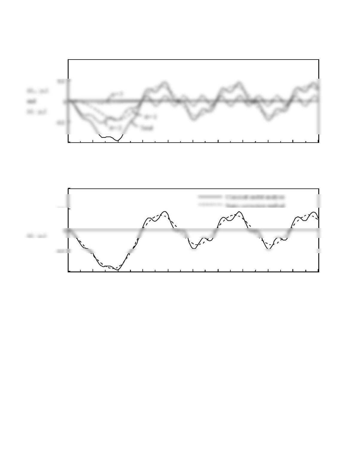
Fig. P12.24a
Figure P12.24b
Figure P12.24a