
The problems in this chapter focus on competitive supply behavior in both the short and long
runs. For short-run analysis, students are usually asked to construct the industry supply curve (by
summing firms’ marginal cost curves) and then to describe the resulting market equilibrium. The
long-run problems (12.4–12.7), on the other hand, make extensive use of the equilibrium
condition P = MC = AC to derive results. In most cases, students are asked to graph their
solutions because such graphs provide considerable intuition about what is going on. The
analytical problems here mainly involve taxation. Problem 12.9 shows that many of the results
for per-unit taxes introduced in the chapter carry over for ad valorem taxes. Problem 12.10
introduces the Ramsey formula for optimal taxation.
Comments on Problems
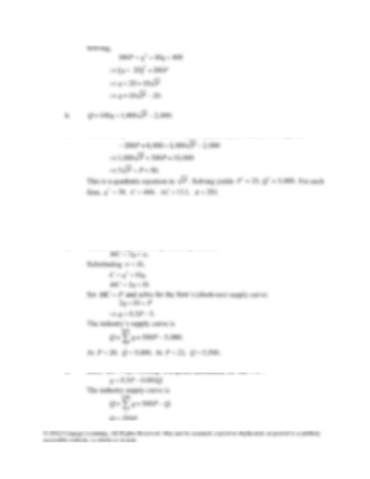
12.1 This problem asks students to construct a marginal cost function from a cubic cost
function and use this to derive a supply curve and a supply–demand equilibrium. The
math is rather easy, so this is a good starting problem.
12.2 This problem illustrates “interaction effects.” As industry output expands, the wage for
diamond cutters rises, thereby raising costs for all firms.
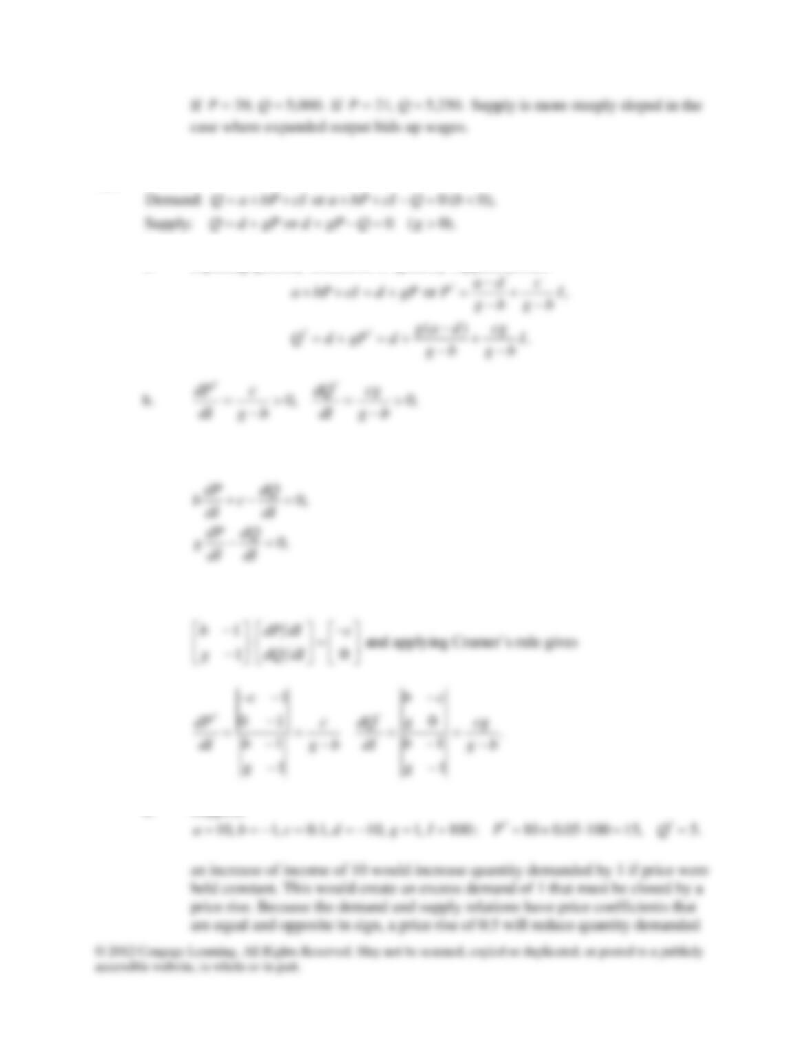
12.3 This problem shows that, with simple linear demand and supply curves, equilibrium
solutions can be found either through substitution or through the comparative statics
procedures illustrated in the chapter.
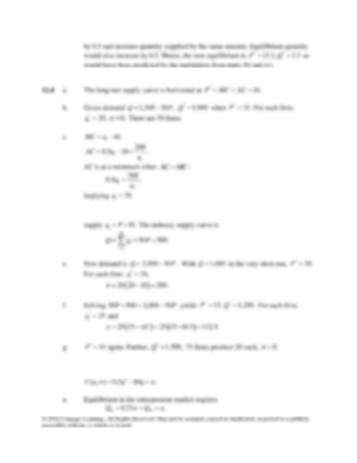
12.4 This is a simple problem in the interaction between short-run and long-run analysis. The
long-run equilibrium price is always $10. But the price may diverge from this in the short
run.
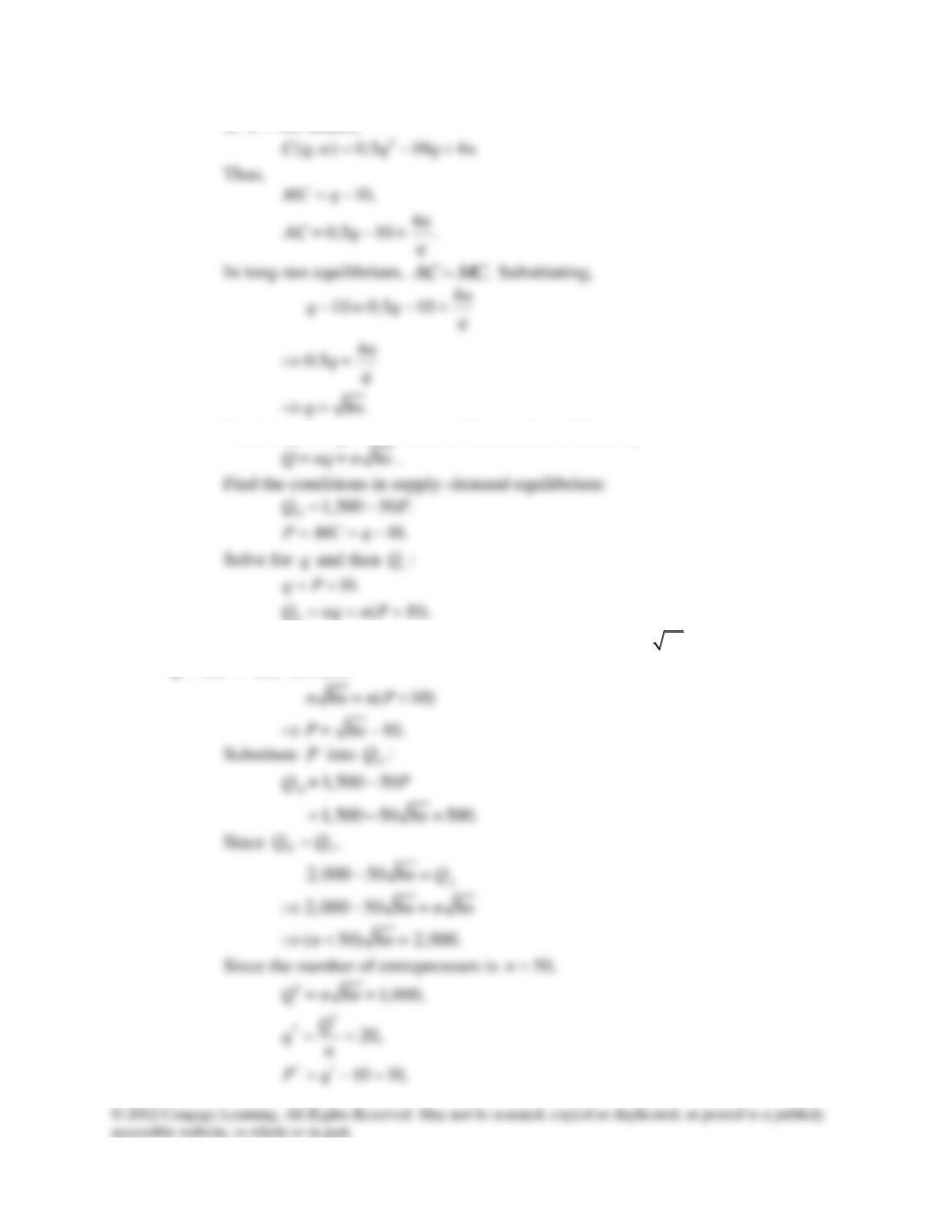
12.5 This problem introduces the concept of increasing input costs into long-run analysis by
assuming that entrepreneurial wages are bid up as the industry expands. Solving part (b)
can be a bit tricky; perhaps an educated guess is the best way to proceed.
12.6 This is a problem in (short-run) tax incidence. The final part of the problem concerns the
change in short-run producer surplus as a result of the tax.
12.7 This is a problem in long-run producer surplus. It makes the point that the producer’s
share of any tax is ultimately borne by that input that is in inelastic supply. Here, it is the
film studio that incurs all of the producer’s share of the tax burden.
CHAPTER 12:
The Partial Equilibrium Competitive Model

12.8 This is a simple partial equilibrium problem in trade theory.
12.9 A simple algebraic model that shows how general parameters for the demand curve and
firms’ cost curves interact to determine the equilibrium price.
Analytical Problems
12.10 Ad valorem taxes . This problem shows that the comparative statics results for ad
valorem taxes are very similar to the results for per-unit taxes shown in Chapter 12. The
problem provides another illustration of why the comparative statics approach taken here
is useful.
12.11 The Ramsey formula for optimal taxation . This problem shows how to compute
optimal rates of ad valorem taxation that minimize the excess burden of these taxes
subject to a total revenue constraint.
12.12 The Cobweb model . This is a simple algebraic model where a lagged supply response
leads to fluctuating prices.
12.13 More on the comparative statics of supply and demand . This exercise contains three
subproblems. The first just asks the student to repeat the analysis in the chapter for a shift
in supply rather than demand. The second examines the effects of a “quantity wedge.”
This yields results very similar to the “tax wedge” analysis in the chapter. Finally, the
problem provides a brief introduction to the identification problem in econometrics as
applied to models of supply and demand.
12.14 The Le Chatelier principle . This introduces Samuelson’s Le Chatelier principle, which
in the supply–demand context simply, shows that any effect of a shift in demand on
prices may set in motion forces (i.e., entry) that tend to reduce the initial price increase.
Such moderation does not operate in the quantity dimension where initial effects become
larger over time.
Solutions
12.1 Given the cost function
Differentiating,
Chapter 12: The Partial Equilibrium Competitive Model
133
c. Demand is
200 8,000.QP= − +
Equating quantity demanded and supplied,
12.2 Given the cost function
2.C q wq=+
a. Differentiating total cost gives marginal cost:
b. Here,
Chapter 12: The Partial Equilibrium Competitive Model
134
12.3
a. Equating quantity demanded to quantity supplied yields:
c. Differentiation of the demand and supply equations yields:
Putting this into matrix notation:
d. Suppose
Chapter 12: The Partial Equilibrium Competitive Model
135
d. The profit-maximization condition is
10.
i
P MC q= = −
Rearranging yields firm
12.5 Given cost function
Chapter 12: The Partial Equilibrium Competitive Model
136
or
4.wn=
Hence,
Total output is given in terms of the number of firms by
S
You are left with three equations in
,Q
,n
.P
Since
8Q = n n
and
( 10),Q n P=+
we have
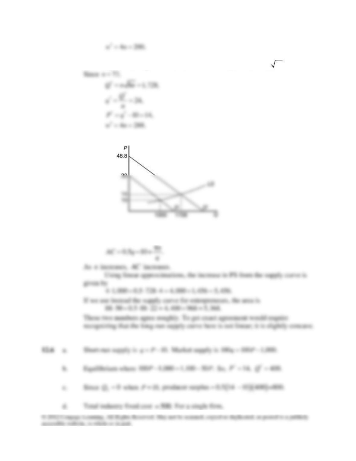
Chapter 12: The Partial Equilibrium Competitive Model
137
b. Following the same algebraic calculations as before yields
( 50) 8 2,928.nn+=
c.
curves shift up:
Chapter 12: The Partial Equilibrium Competitive Model
138
e. With tax,
3.
DS
PP=+
Equating supply and demand,
Chapter 12: The Partial Equilibrium Competitive Model
139
d. The change in rents is
e. With tax,
5.5.
DS
PP=+
Supply is
10 .002 .
S
PQ=+
In terms of the consumer
f. CS originally
( )( )
0.5 500 21 11 2,500.= − =
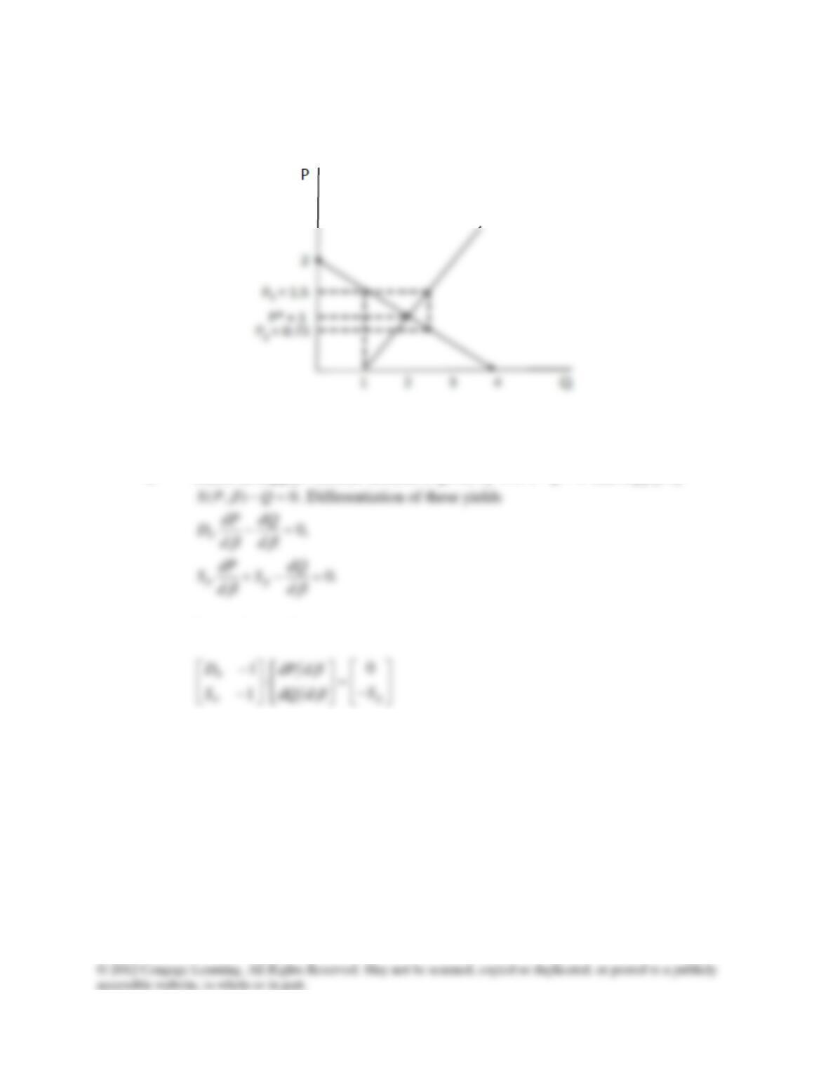
12.8 a. Solve
150 5,000 100PP=−
for domestic equilibrium. This yields
*20,P=
* 4,000.
D
Q=
c. If price rises to 15,
* 3,500.
D
Q=
Chapter 12: The Partial Equilibrium Competitive Model
140
d. With quota of 1,250, results duplicate part (c) except no tariff revenues are
12.9 a. Long-run equilibrium requires P = AC = MC.
b. Want supply = demand
)2( kbaBABPA
b
k
nnq +−=−==
Analytical Problems
12.10. Ad valorem taxes
a.
dP dQ dP dQ
Chapter 12: The Partial Equilibrium Competitive Model
141
b.
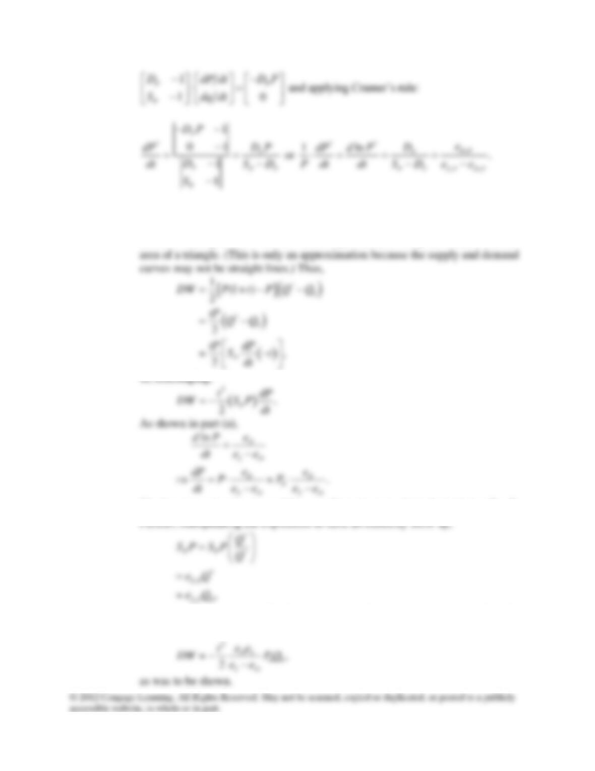
DW
is given as the area of the shaded region in the graph below. For a small tax
increase starting from
0,t=
DW
can be approximated using the formula for the
The last approximation is good for a small tax increase above 0, implying
0.PP
where the approximation
*0
QQ
is again good for a small tax increase above 0.
Substituting these results into the expression for
,DW
Chapter 12: The Partial Equilibrium Competitive Model
142
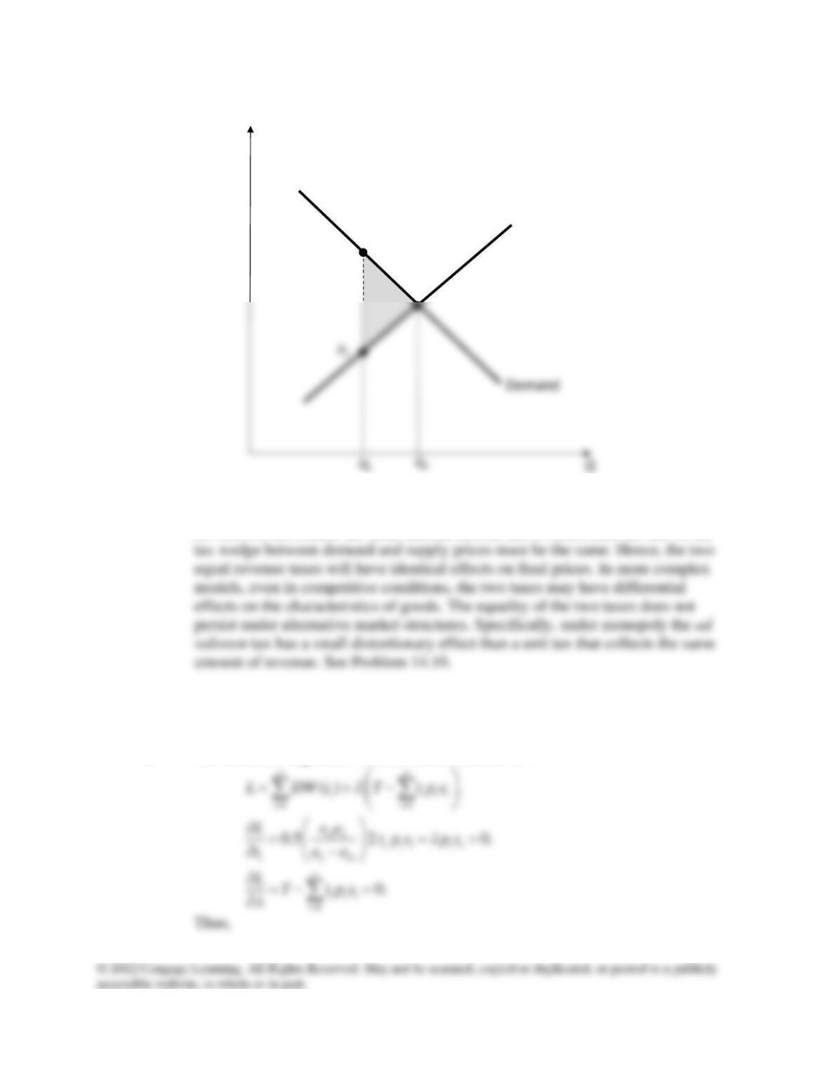
c. Under perfect competition the tax “wedge” diagram shows that if a unit tax and an
ad valorem tax collect the same amount in total tax revenue, then the size of the
12.11 The Ramsey formula for optimal taxation
a. Use the deadweight loss formula from Problem 12.9:
P
Supply
PS (1+t)
Chapter 12: The Partial Equilibrium Competitive Model
143
b. The above formula suggests that higher taxes should be applied to goods with
c. This result was obtained under a set of very restrictive assumptions. First, it was
12.12 Cobweb models
b.
c. Repeated substitution yields
d. Use
So,
Chapter 12: The Partial Equilibrium Competitive Model
144
12.13 More on the comparative statics of supply and demand
a. Shifts in supply: Assume demand is given by
( ) 0D P Q−=
and supply by
In matrix notation
And Cramer’s rule shows that
Chapter 12: The Partial Equilibrium Competitive Model
145
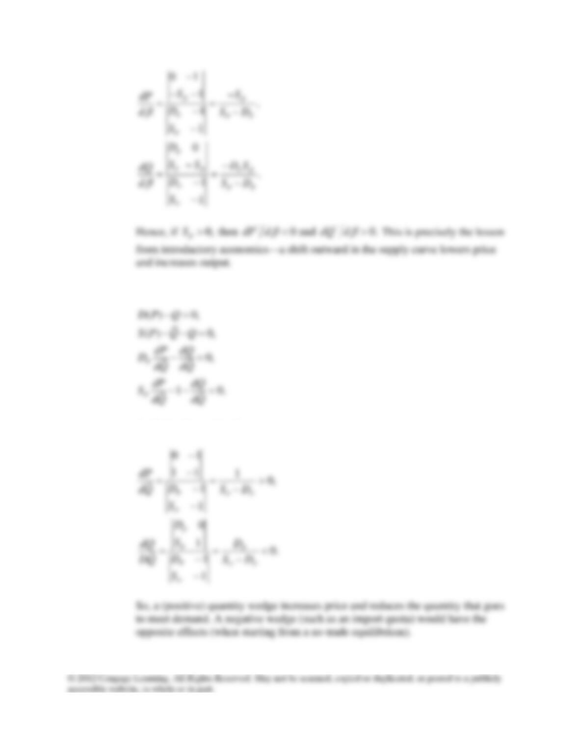
b. A quantity wedge
Applying Cramer’s rule
Chapter 12: The Partial Equilibrium Competitive Model
146
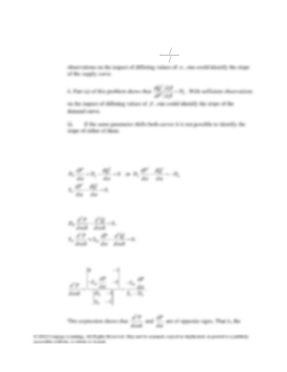
c. The identification problem
i. The analysis in the chapter shows that
*
*P
dQ d S
dP d
=
. With sufficient
12.14 The Le Chatelier Principle
a. Here are Equations 12.24:
Differentiation with respect to t yields
b. Cramer’s rule can now be used to solve for the second-order partials:
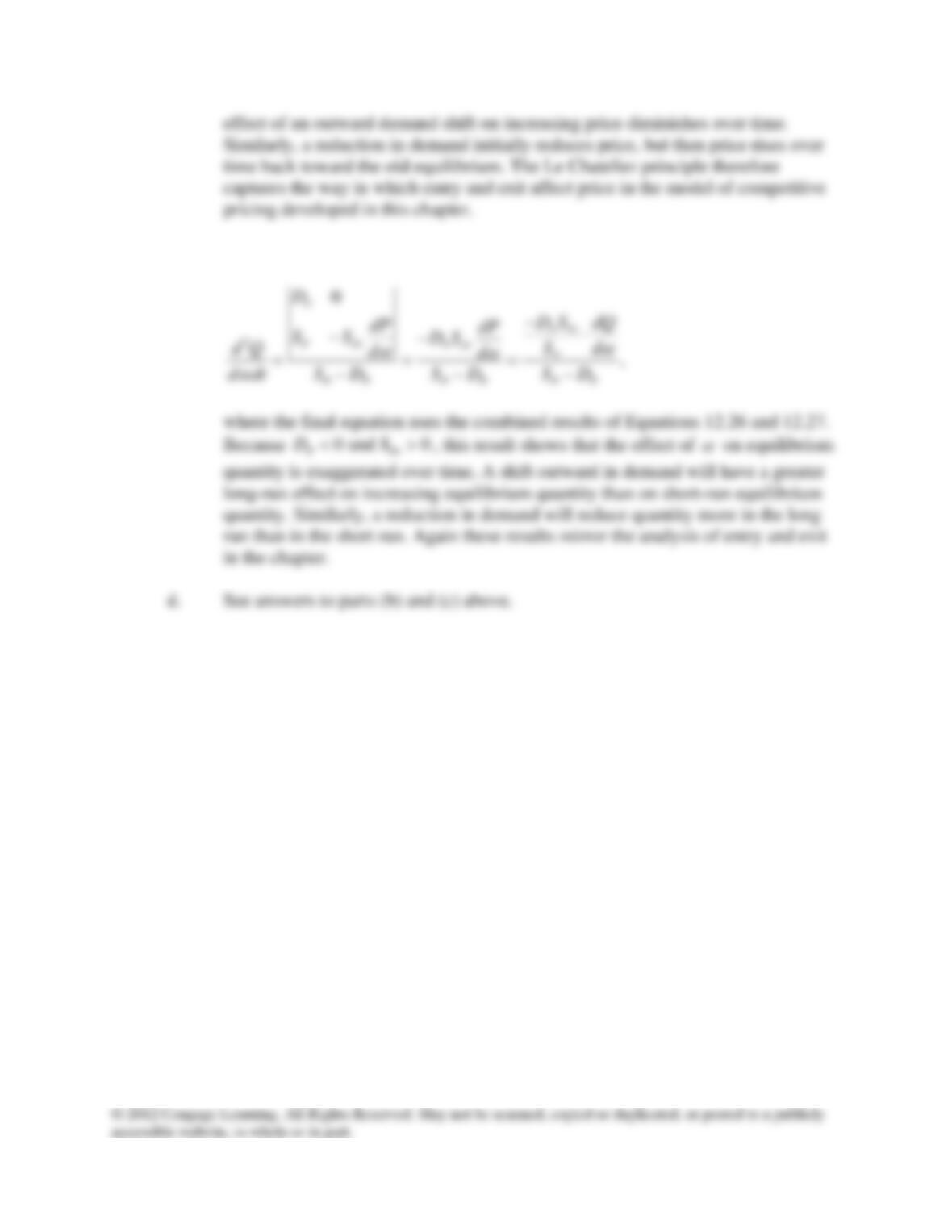
Chapter 12: The Partial Equilibrium Competitive Model
147
c. Again, we use Cramer’s rule: