Chapter 12 Homework Plot Pxy diagram with fit and data γ1x1x2

γ1x1x2,()

exp x2

Λ12

x1 x2 Λ12

⋅+

Λ21

x2 x1 Λ21

⋅+

−

⎛

⎜

⎝

⎞

⎠

⋅

⎡

⎢

⎣

⎤

⎥

⎦

x1 x2 Λ12

⋅+

()

:=

⎜

⎢

⎥

Λ21

⎛

⎞

⎡

⎤

394

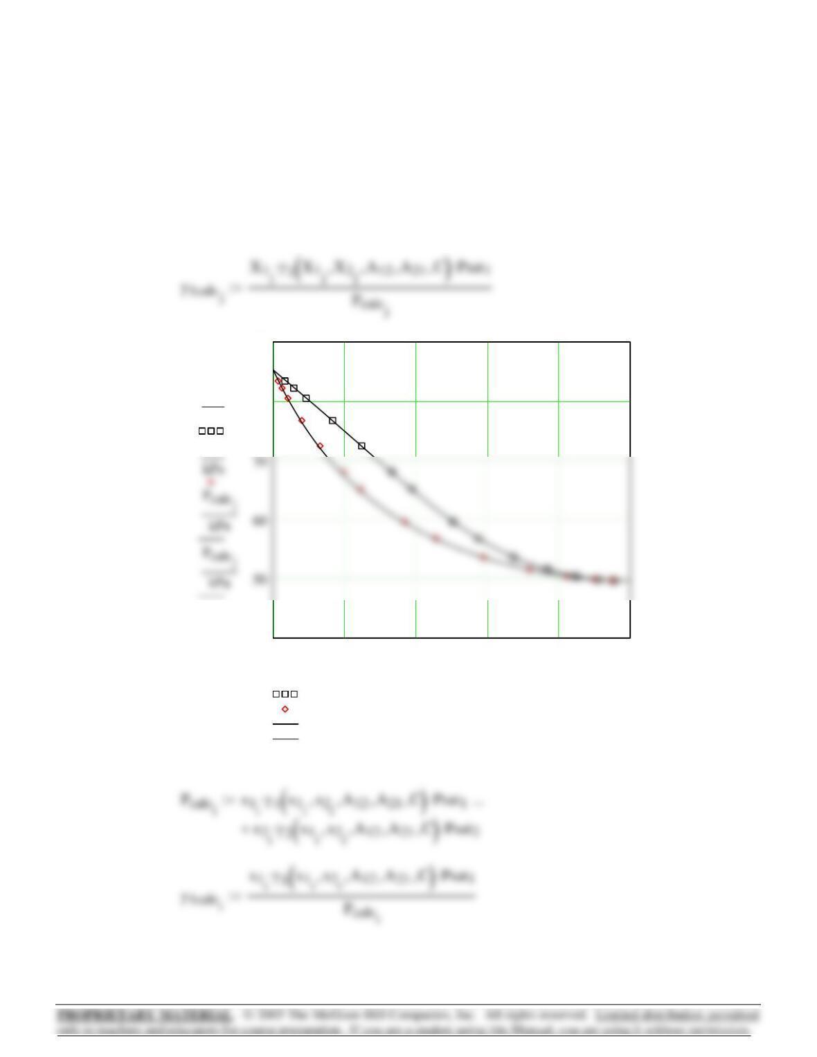
P-x,y diagram: Wilson eqn. fit to GE/RT data.

0 0.2 0.4 0.6 0.8 1

65

100

105

P-x data

Pi

x1iy1i

,X1j

,Y1calcj

,

RMS deviation in P:

RMS

i

PiPcalci

−

()

2

n

∑

:= RMS 0.361 kPa=

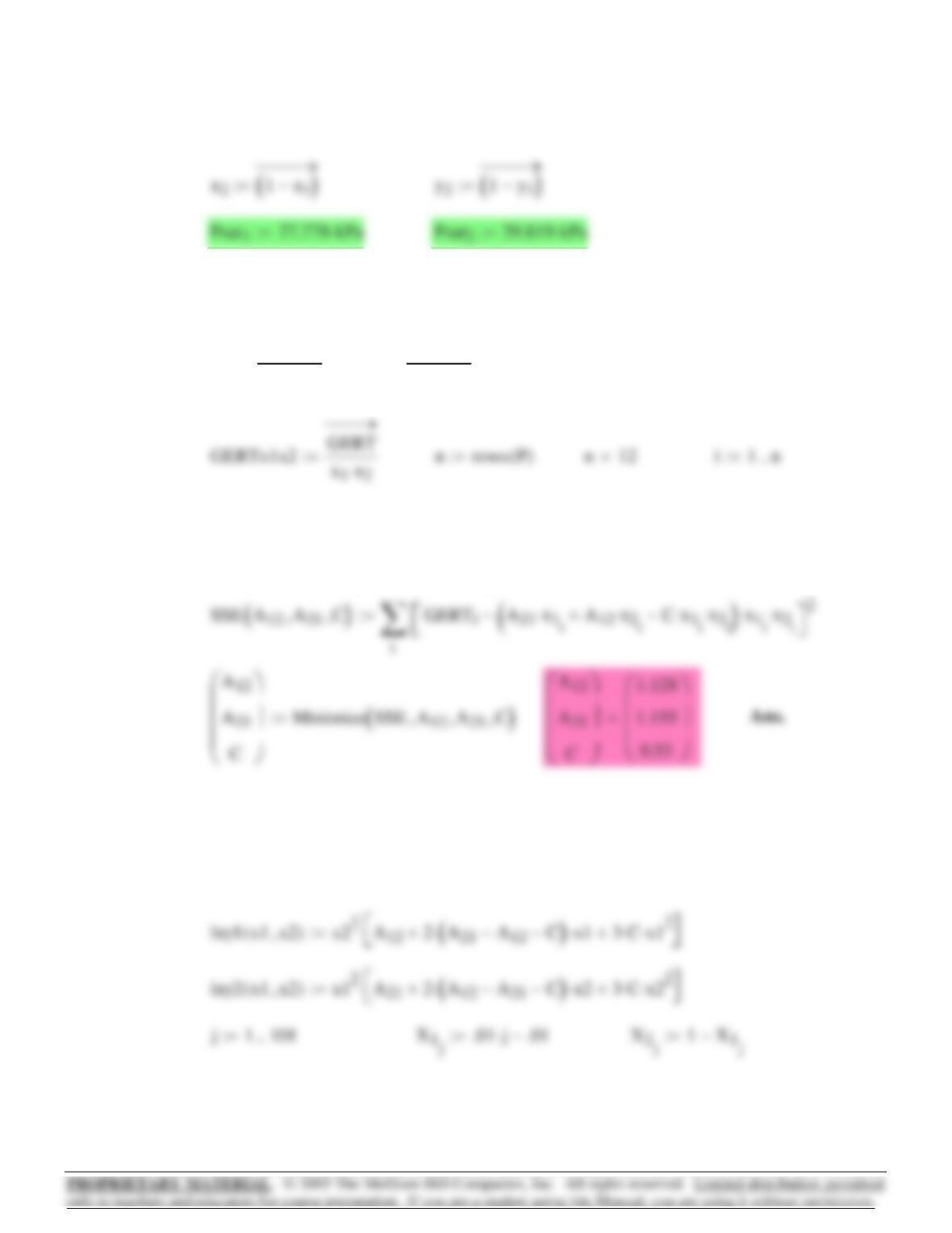
(d) BARKER’S METHOD by non-linear least squares.

Margules equation.

Guesses for parameters: answers to Part (a).

γ1x1 x2,A12

,A21

,

()

exp x2()

2A12 2A

21 A12

−

()

⋅x1⋅+

⎡

⎣

⎤

⎦

⋅

⎡

⎣

⎤

⎦

:=

γ2x1 x2,A12

,A21

,

()

exp x1()

2A21 2A

12 A21

−

()

⋅x2⋅+

⎡

⎣

⎤

⎦

⋅

⎡

⎣

⎤

⎦

:=

395

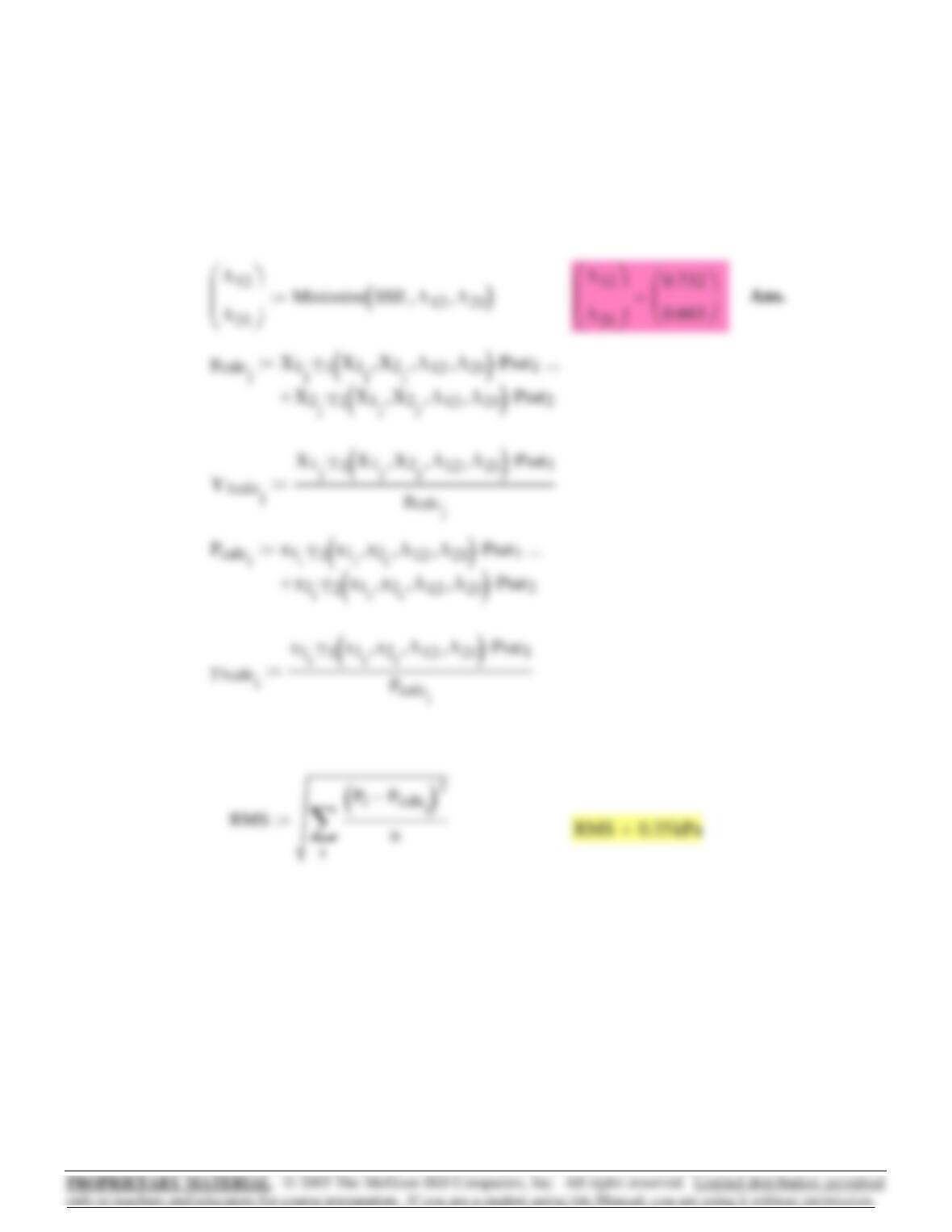
RMS 0.365 kPa=RMS

i

PiPcalci

−

()

2

n

∑

:=

RMS deviation in P:

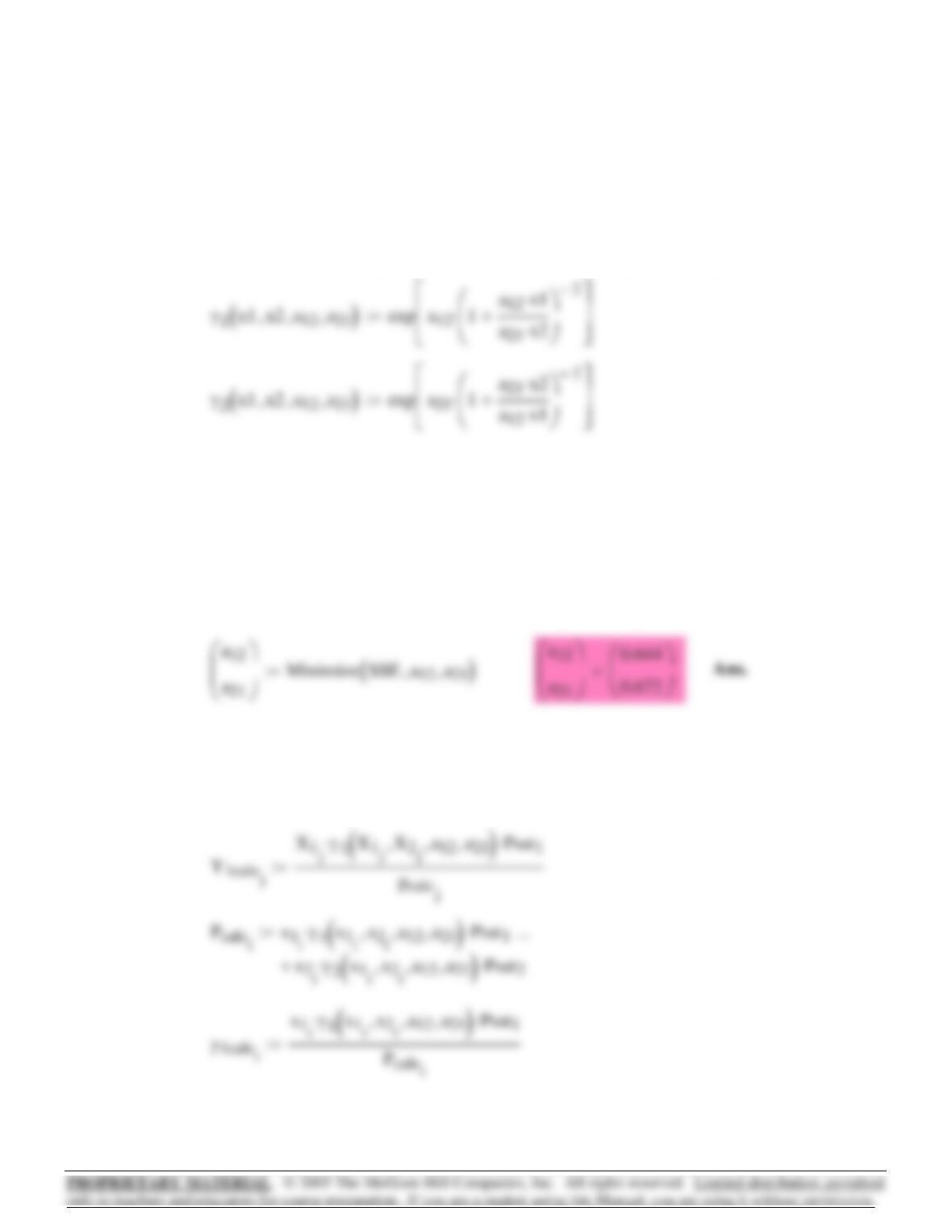
pcalcjX1jγ1X1jX2j

,A12

,A21

,

()

⋅Psat1

⋅

X2jγ2X1jX2j

,A12

,A21

,

()

⋅Psat2

⋅+

…:=

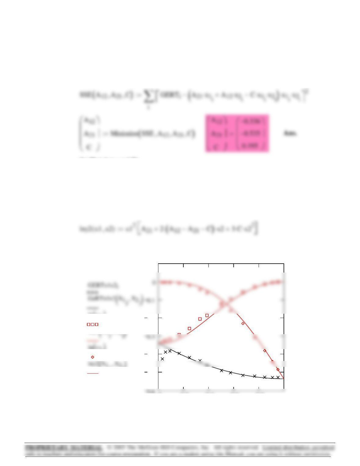
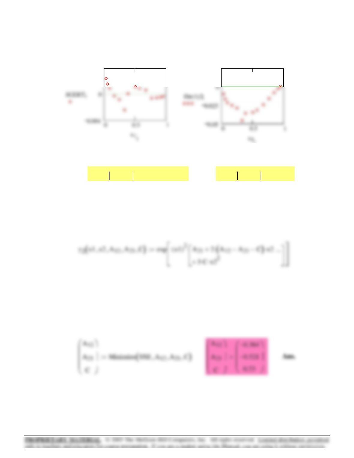
SSE A12 A21

,

()

i

Pix1iγ1x1ix2i

,A12

,A21

,

()

⋅Psat1

⋅

x2iγ2x1ix2i

,A12

,A21

,

()

⋅Psat2

⋅+

…

⎛

⎜

⎝

⎞

⎠

−

⎡

⎢

⎣

⎤

⎥

⎦

2

∑

:=

A21 1.0:=A12 0.5:=

Guesses:

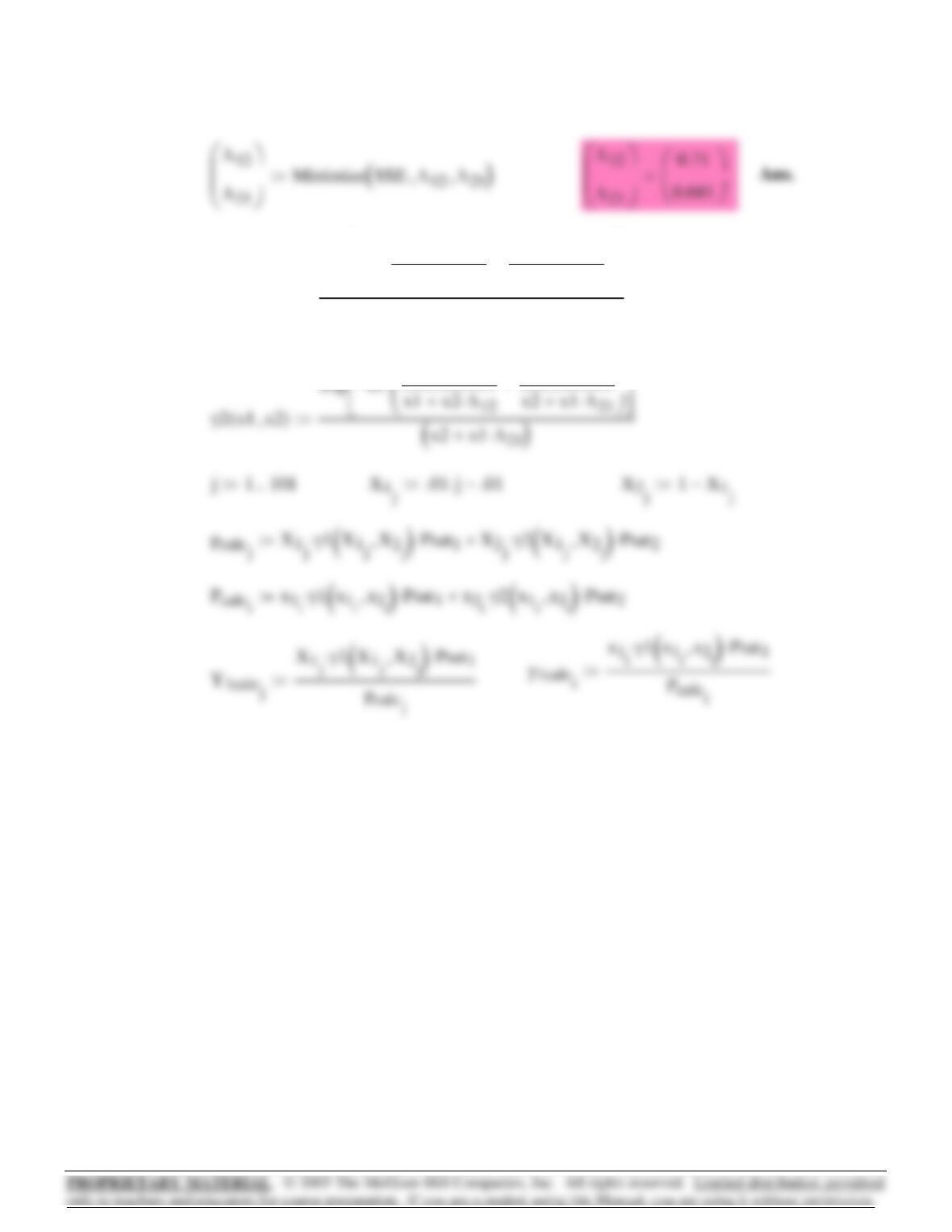
Minimize the sum of the squared errors using the Mathcad Minimize function.

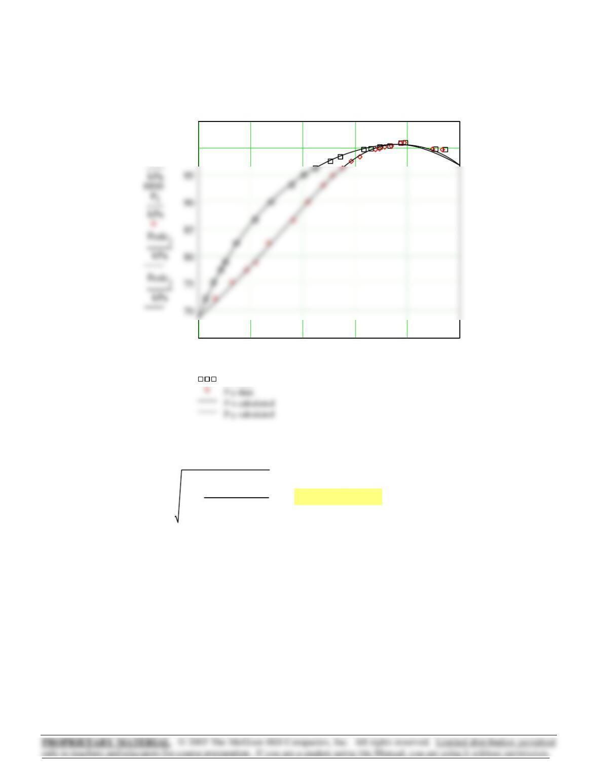
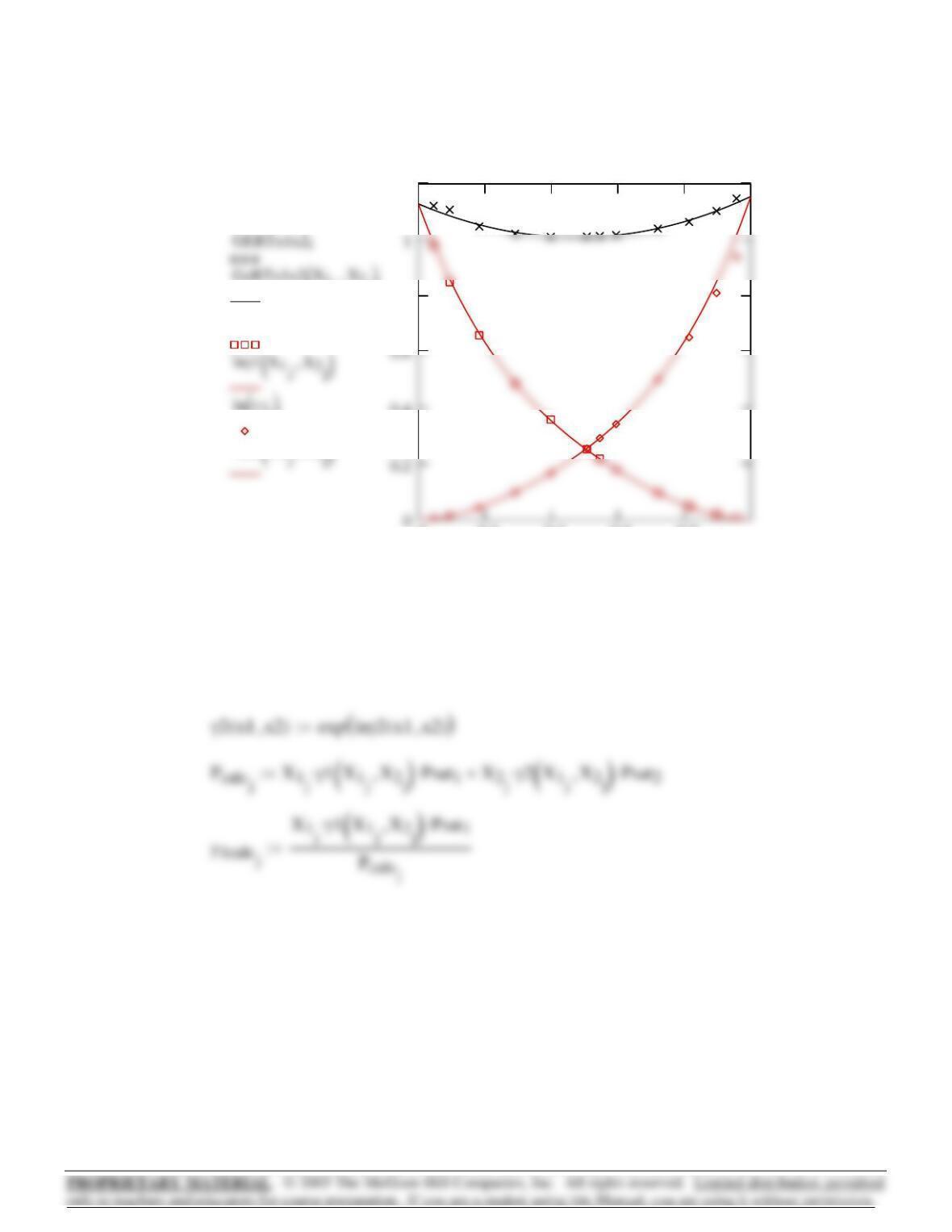
396

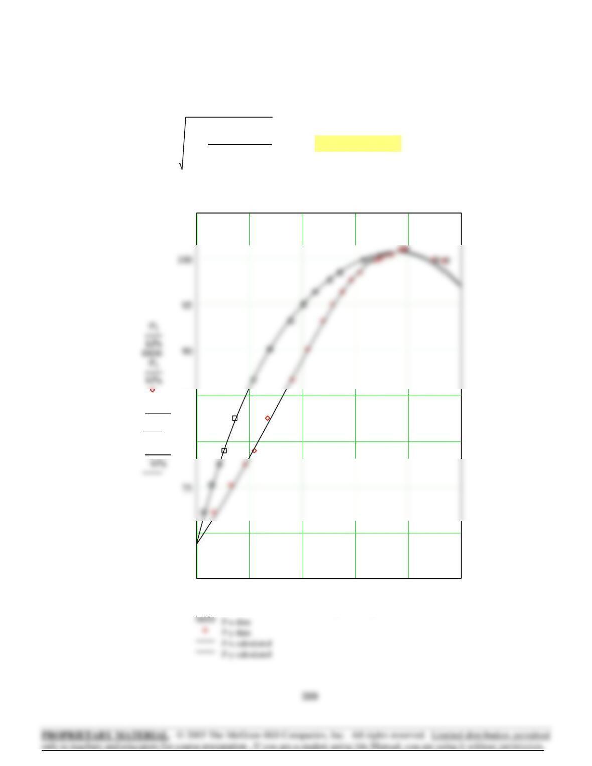
P-x-y diagram, Margules eqn. by Barker’s method

0 0.2 0.4 0.6 0.8 1

65

100

105

P-x data

P-y data

P-x calculated

P-y calculated

Pi

x1iy1i

,X1j

,Y1calcj

,

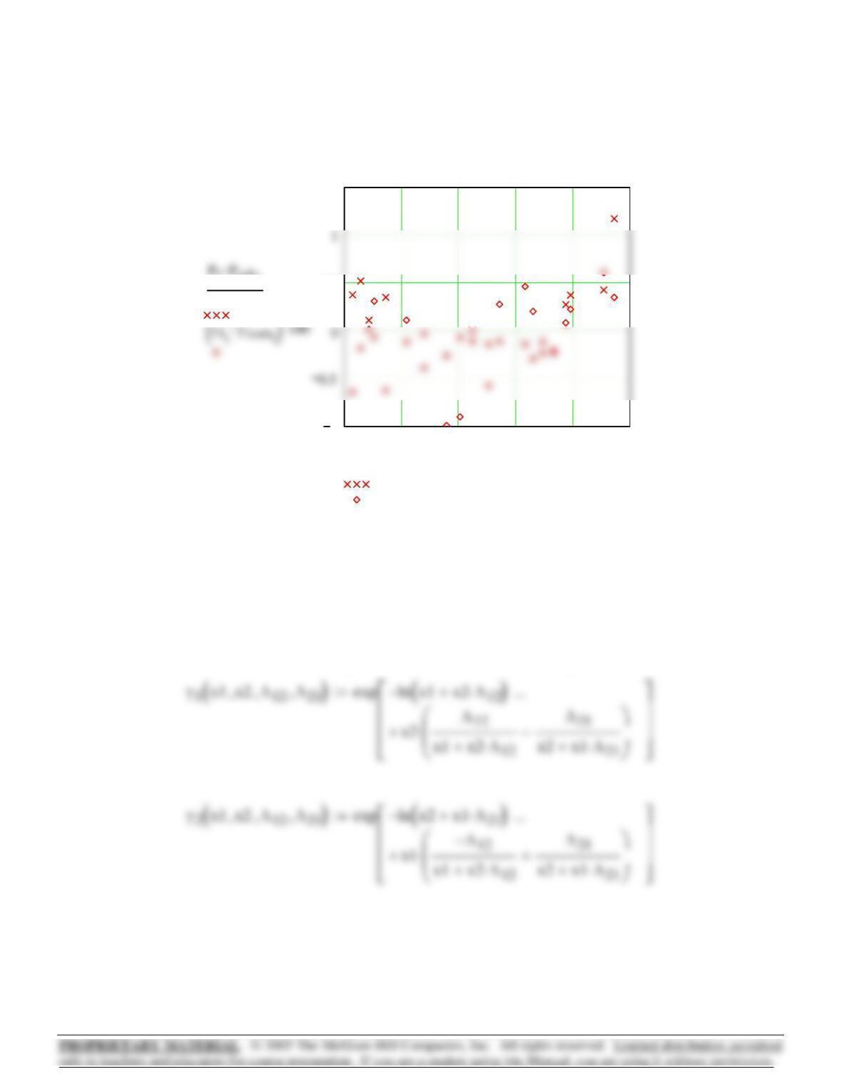
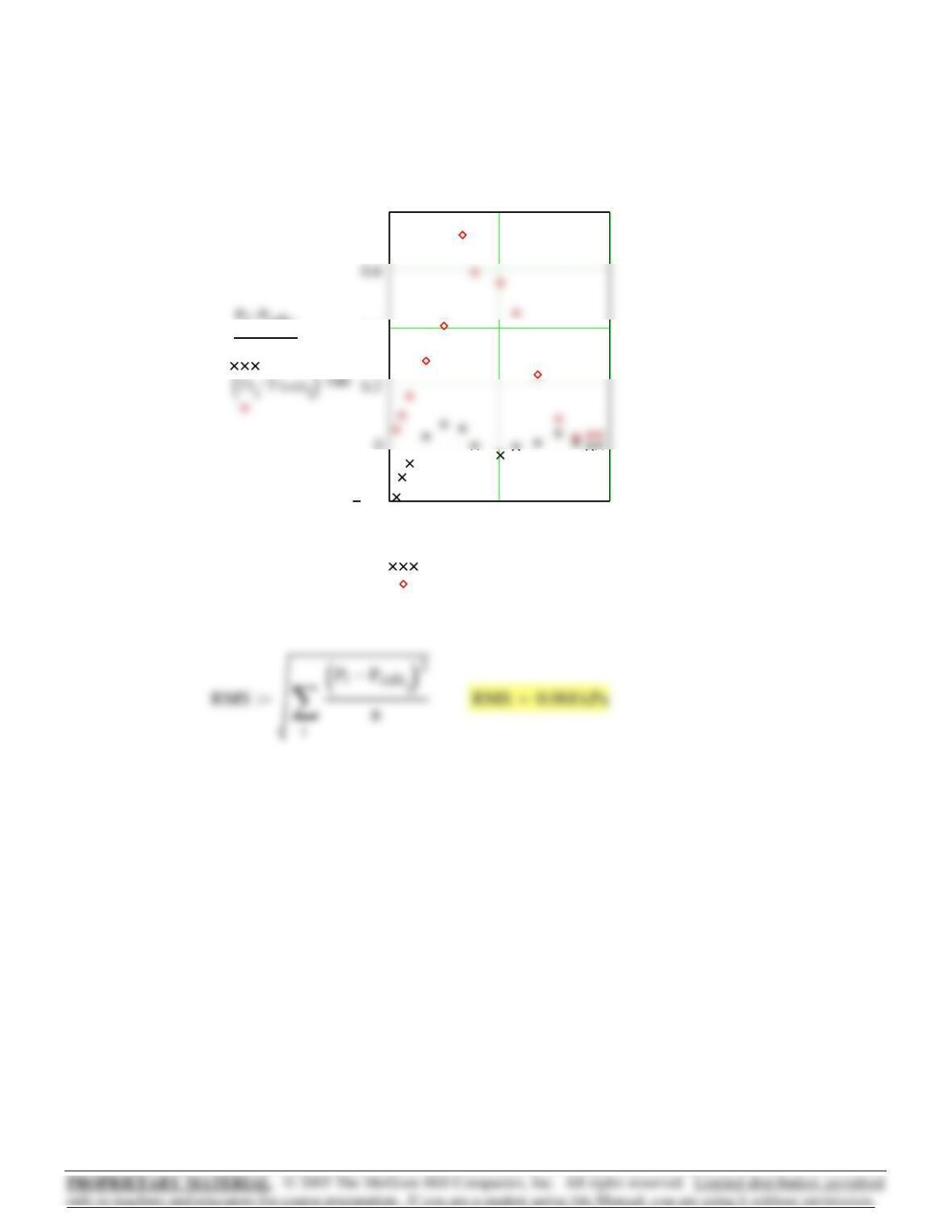
Residuals in P and y1

2

397

pcalcjX1jγ1X1jX2j

,a12

,a21

,

()

⋅Psat1

⋅

X2jγ2X1jX2j

,a12

,a21

,

()

⋅Psat2

⋅+

…:=

SSE a12 a21

,

()

i

Pix1iγ1x1ix2i

,a12

,a21

,

()

⋅Psat1

⋅

x2iγ2x1ix2i

,a12

,a21

,

()

⋅Psat2

⋅+

…

⎛

⎜

⎝

⎞

⎠

−

⎡

⎢

⎣

⎤

⎥

⎦

2

∑

:=

a21 1.0:=a12 0.5:=

Guesses:

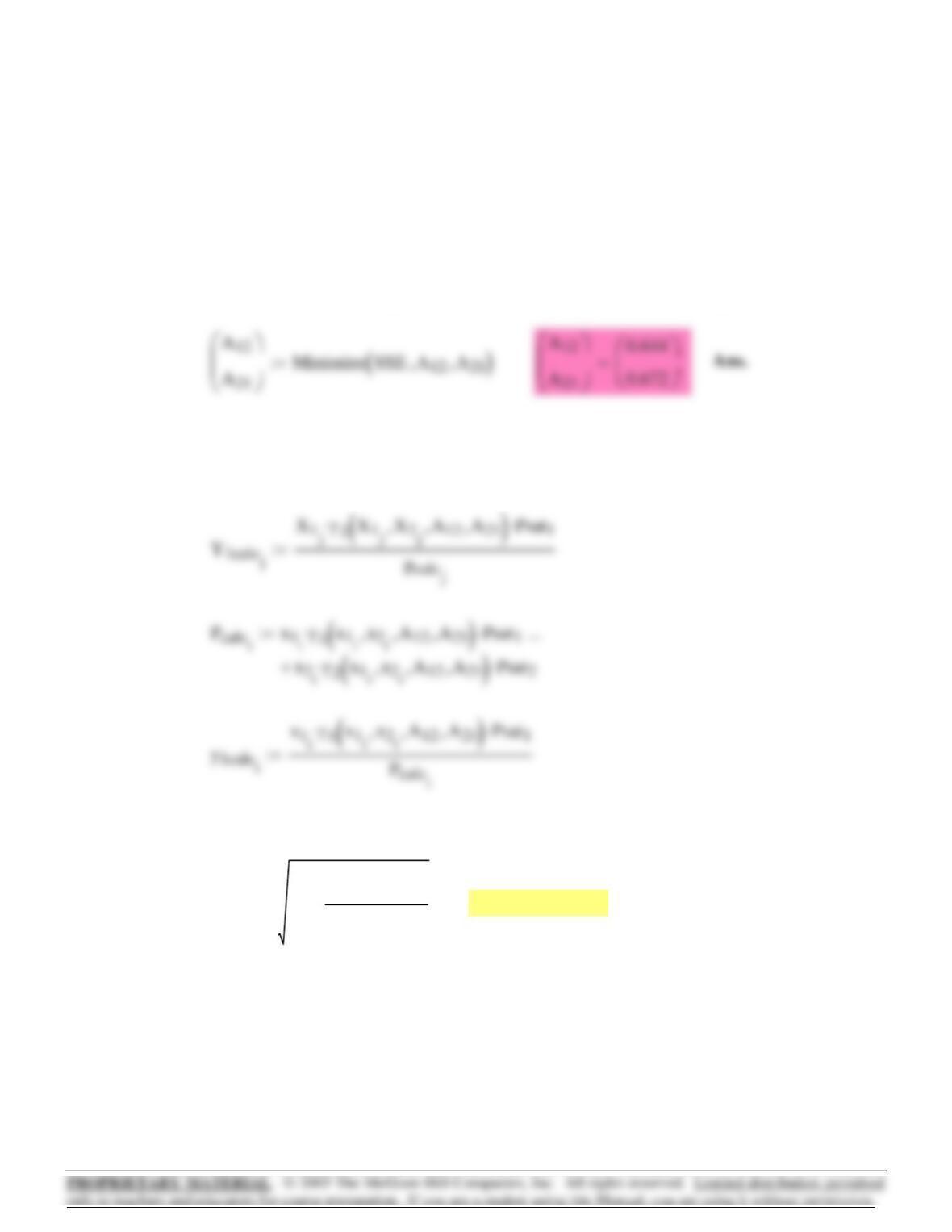
Minimize the sum of the squared errors using the Mathcad Minimize function.

⎢

⎥

⎢

⎥

j 1 101..:= X2j1X

1j

−:=X1j.01 j⋅.00999−:=

Guesses for parameters: answers to Part (b).

BARKER’S METHOD by non-linear least squares.

van Laar equation.

(e)

398

RMS deviation in P:

RMS

i

PiPcalci

−

()

2

n

∑

:= RMS 0.364 kPa=

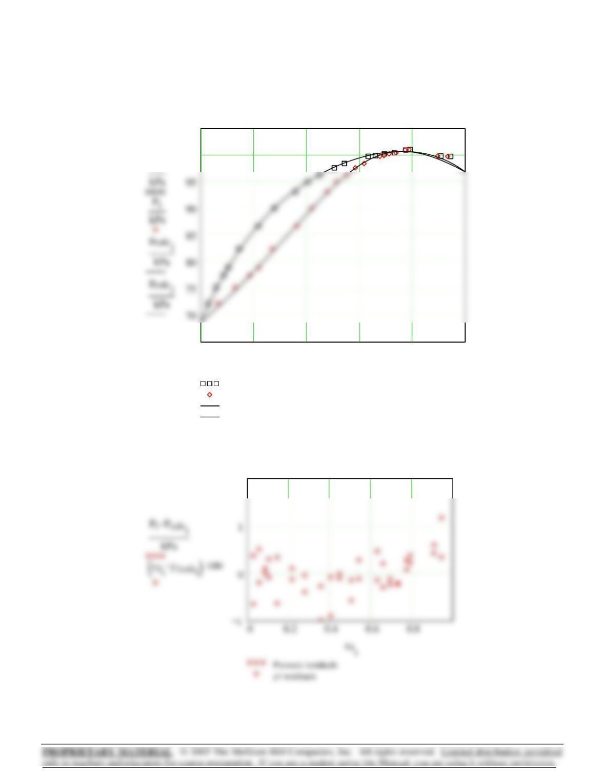
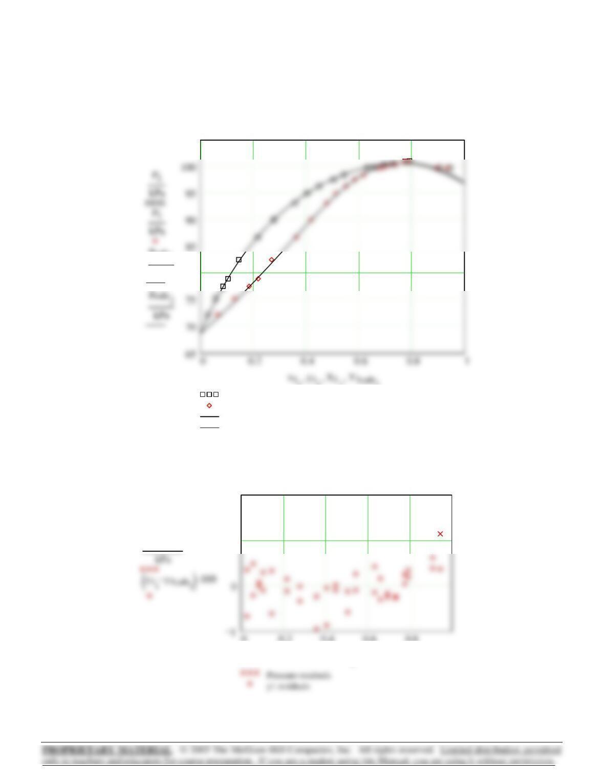
P-x,y diagram, van Laar Equation by Barker’s Method

0 0.2 0.4 0.6 0.8 1

65

70

80

85

105

pcalcj

kPa

pcalcj

x1iy1i

,X1j

,Y1calcj

,

Λ21 1.0:=Λ12 0.5:=

Guesses:

Minimize the sum of the squared errors using the Mathcad Minimize function.

X2j1X

1j

−:=X1j.01 j⋅.01−:=j 1 101..:=

Guesses for parameters: answers to Part (c).

Wilson equation.

BARKER’S METHOD by non-linear least squares.(f)

0 0.2 0.4 0.6 0.8

1

0.5

1.5

Pressure residuals

y1 residuals

kPa

x1i

Residuals in P and y1.

400

SSE Λ12 Λ21

,

()

i

Pix1iγ1x1ix2i

,Λ

12

,Λ

21

,

()

⋅Psat1

⋅

x2iγ2x1ix2i

,Λ

12

,Λ

21

,

()

⋅Psat2

⋅+

…

⎛

⎜

⎝

⎞

⎠

−

⎡

⎢

⎣

⎤

⎥

⎦

2

∑

:=

RMS deviation in P:

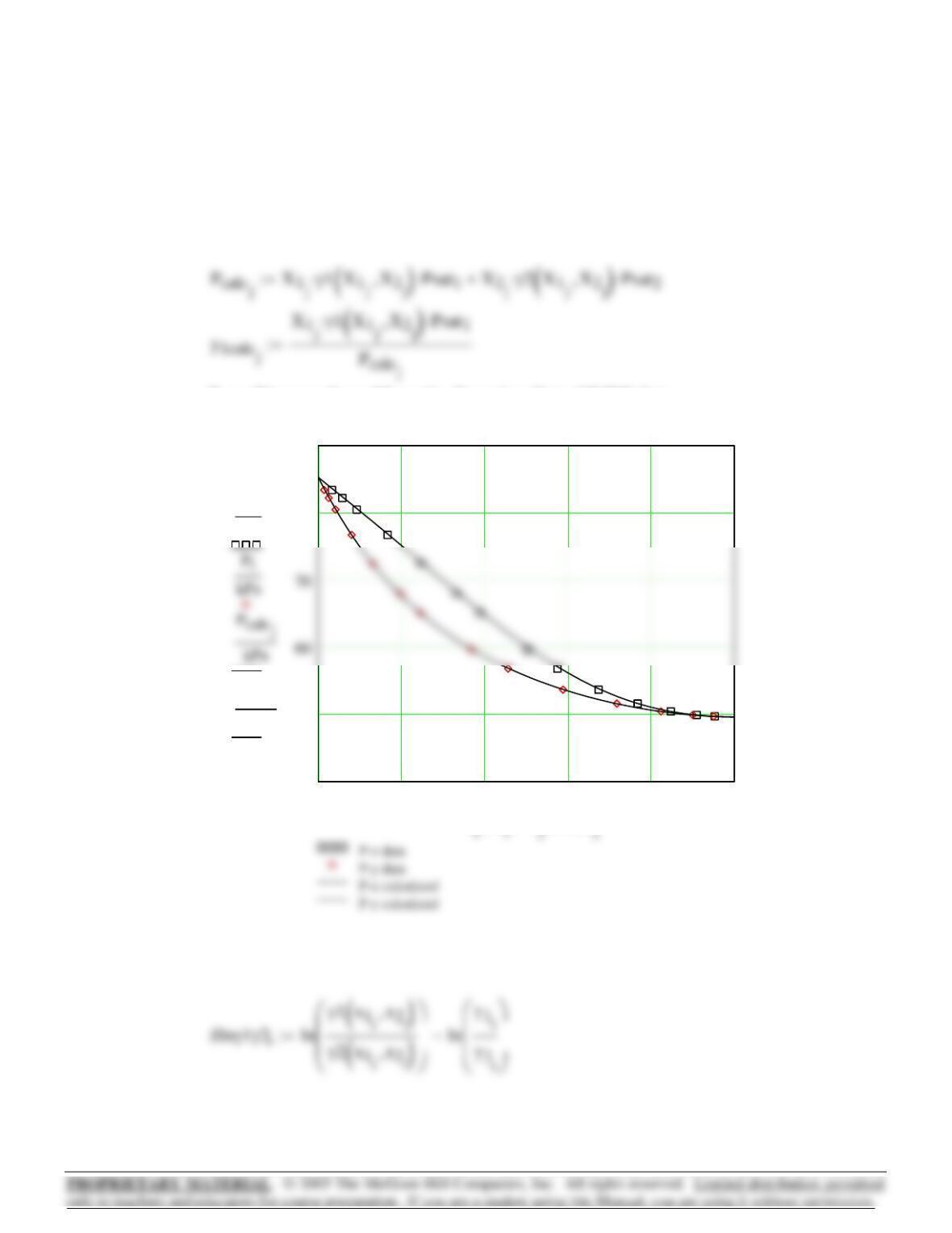
401

⎜

P-x,y diagram, Wilson Equation by Barker’s Method

80

105

P-x data

P-y data

P-x calculated

P-y calculated

pcalcj

kPa

Residuals in P and y1.

0 0.2 0.4 0.6 0.8

1

2

PiPcalci

−

x1i

402

i1n..:=n14=n rows P():=GERTx1x2 GERT

x1x2

⋅

→

⎯

:=

GERT x1ln γ1

()

⋅x2ln γ2

()

⋅+

()

→

⎯

⎯⎯⎯⎯⎯⎯⎯

⎯

:=γ2

y2P⋅

x2Psat2

⋅

→

⎯

:=γ1

y1P⋅

x1Psat1

⋅

→

⎯

:=

Calculate EXPERIMENTAL values of activity coefficients and excess

Gibbs energy.

Psat285.265 kPa⋅:=Psat149.624 kPa⋅:=

y21y

1

−

()

→

⎯

:=x21x

1

−

()

→

⎯

:=

y1

0.0141

0.0253

0.0416

0.0804

0.1314

0.1975

0.2457

0.3686

0.4564

0.5882

0.7176

0.8238

0.9002

0.9502

⎛

⎜

⎝

⎞

⎟

⎠

:=

x1

0.0330

0.0579

0.0924

0.1665

0.2482

0.3322

0.3880

0.5036

0.5749

0.6736

0.7676

0.8476

0.9093

0.9529

⎛

⎜

⎝

⎞

⎟

⎠

:=

P

83.402

82.202

80.481

76.719

72.442

68.005

65.096

59.651

56.833

53.689

51.620

50.455

49.926

49.720

⎛

⎜

⎝

⎞

⎟

⎠

kPa⋅:=

T 308.15 K⋅:=

Methyl t-butyl ether(1)/Dichloromethane–VLE data:12.6

403

0 0.2 0.4 0.6 0.8

0.5

0.4

0.2

ln γ1i

()

lnγ1X

,

()

x1iX1j

,x1i

,X1j

,x1i

,X1j

,

X2j1X

1j

−:=X1j.01 j⋅.01−:=j 1 101..:=

⎡

⎣

⎤

⎦

lnγ1x1x2,()x2

2A12 2A

21 A12

−C−

()

⋅x1⋅+ 3C⋅x12

⋅+

⎡

⎣

⎤

⎦

⋅:=

GeRT x1 x2,( ) GeRTx1x2 x1 x2,()x1⋅x2⋅:=

GeRTx1x2 x1 x2,()A

21 x1⋅A12 x2⋅+ Cx1⋅x2⋅−

()

:=

(b) Plot data and fit

⎜

⎡

⎣

⎤

⎦

C 0.2:=A21 0.5−:=A12 0.3−:=

Guesses:

Minimize sum of the squared errors using the Mathcad Minimize function.

Fit GE/RT data to Margules eqn. by nonlinear least squares.(a)

404

(c) Plot Pxy diagram with fit and data

γ1x1x2,( ) exp lnγ1x1x2,()

()

:=

γ2x1x2,( ) exp lnγ2x1x2,()

()

:=

P-x,y Diagram from Margules Equation fit to GE/RT data.

0 0.2 0.4 0.6 0.8

40

50

80

90

Pi

kPa

Pcalcj

kPa

x1iy1i

,X1j

,y1calcj

,

(d) Consistency Test: δGERTiGeRT x1ix2i

,

()

GERTi

−:=

405

SSE A12 A21

,C,

()

i

Pix1iγ1x1ix2i

,A12

,A21

,C,

()

⋅Psat1

⋅

x2iγ2x1ix2i

,A12

,A21

,C,

()

⋅Psat2

⋅+

…

⎛

⎜

⎝

⎞

⎠

−

⎡

⎢

⎣

⎤

⎥

⎦

2

∑

:=

C 0.2:=A21 0.5−:=A12 0.3−:=

Guesses:

Minimize sum of the squared errors using the Mathcad Minimize function.

⎢

⎥

⎢

⎥

γ1x1 x2,A12

,A21

,C,

()

exp x2()

2A12 2A

21 A12

−C−

()

⋅x1⋅+

3C⋅x12

⋅+

…

⎡

⎢

⎣

⎤

⎥

⎦

⋅

⎡

⎢

⎣

⎤

⎥

⎦

:=

Barker’s Method by non-linear least squares:

Margules Equation

(e)

mean δlnγ1γ2

→

⎯

⎯⎯

⎯

()

0.021=mean δGERT

→

⎯

⎯⎯

⎯

()

9.391 10 4−

×=

Calculate mean absolute deviation of residuals

0.004

406

⎜

Plot P-x,y diagram for Margules Equation with parameters from Barker’s

Method.

PcalcjX1jγ1X1jX2j

,A12

,A21

,C,

()

⋅Psat1

⋅

X2jγ2X1jX2j

,A12

,A21

,C,

()

⋅Psat2

⋅+

…:=

0 0.2 0.4 0.6 0.8

40

80

90

P-x data

P-y data

P-x calculated

P-y calculated

Pi

kPa

Pi

x1iy1i

,X1j

,y1calcj

,

407

Plot of P and y1 residuals.

0 0.5 1

0.2

0.4

0.8

Pressure residuals

y1 residuals

kPa

x1i

RMS deviations in P:

408

γ1x1x2,( ) exp x22A12 2A

21 A12

−

()

⋅x1⋅+

⎡

⎣

⎤

⎦

⋅

⎡

⎣

⎤

⎦

:=

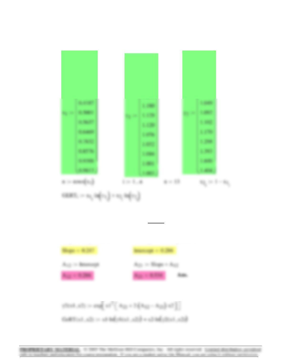
Intercept intercept X Y,():=Slope slope X Y,():=

Yi

GERTi

x1ix2i

⋅

:=Xix1i

:=

Fit GE/RT data to Margules eqn. by linear least-squares procedure:(b)

1.202

1.307

1.295

1.228

1.234

⎛

⎜

⎞

⎟

1.002

1.004

1.006

1.024

1.022

⎛

⎜

⎞

⎟

0.0523

0.1299

0.2233

0.2764

0.3482

⎛

⎜

⎞

⎟

Data:(a)12.8

409

⎡

⎣

⎤

⎦

⎡

⎣

⎤

⎦

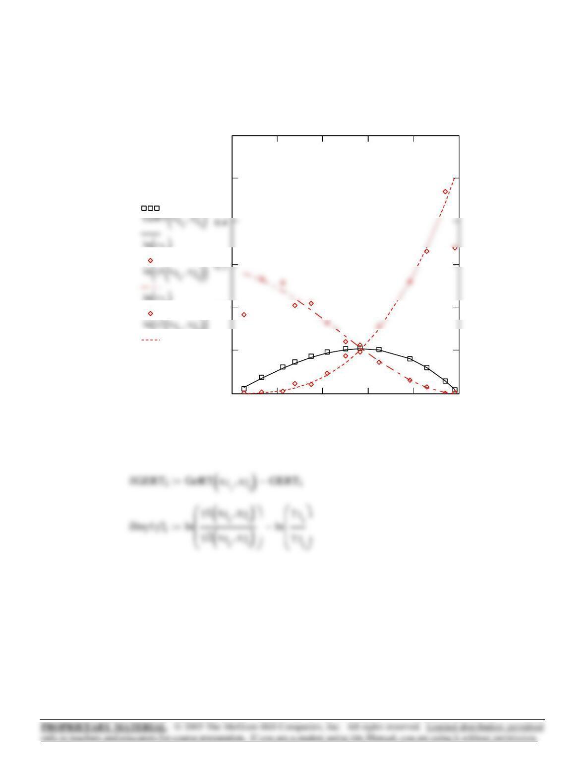
Plot of data and correlation:

0 0.2 0.4 0.6 0.8

0

0.1

0.2

0.5

GERTi

()

x1i

(c) Calculate and plot residuals for consistency test:

410

0 0.5 1

0.1

x1i

δGERTi

-3

3.314·10

-3

-2.998·10

-2.874·10

-3

-2.22·10

-2.174·10

-3

-1.553·10

-8.742·10

-4

2.944·10

5.962·10

9.025·10

4.236·10

=δlnγ1γ2i

0.098

0.026

-0.019

-3

5.934·10

0.028

-3

-9.59·10

9.139·10

-4

-5.617·10

-0.011

0.028

-0.168

=

Calculate mean absolute deviation of residuals:

12.9 Acetonitrile(1)/Benzene(2)– VLE data T 318.15 K⋅:=

P

31.957

35.285

36.996

36.978

35.792

32.331

30.038

⎛

⎜

⎝

⎞

⎟

⎠

0.0455

0.1829

0.3980

0.5458

0.7206

0.8972

0.9573

⎛

⎜

⎝

⎞

⎟

⎠

0.1056

0.2783

0.4274

0.5098

0.6157

0.7869

0.8916

⎛

⎜

⎝

⎞

⎟

⎠

411

GeRT x1 x2,( ) GeRTx1x2 x1 x2,()x1⋅x2⋅:=

GeRTx1x2 x1 x2,()A

21 x1⋅A12 x2⋅+ Cx1⋅x2⋅−

()

:=

(b) Plot data and fit

C 0.2:=A21 0.5−:=A12 0.3−:=

⎯

Calculate EXPERIMENTAL values of activity coefficients and excess

Gibbs energy.

γ1

y1P⋅

x1Psat1

⋅

→

⎯

:= γ2

y2P⋅

x2Psat2

⋅

→

⎯

:= GERT x1ln γ1

()

⋅x2ln γ2

()

⋅+

()

→

⎯

⎯⎯⎯⎯⎯⎯⎯

⎯

:=

⎯

(a) Fit GE/RT data to Margules eqn. by nonlinear least squares.

Minimize sum of the squared errors using the Mathcad Minimize function.

Guesses:

412

0 0.2 0.4 0.6 0.8

0.4

0.8

1.2

()

ln γ1i

()

lnγ2X

1jX2j

,

x1iX1j

,x1i

,X1j

,x1i

,X1j

,

(c) Plot Pxy diagram with fit and data

γ1x1x2,( ) exp lnγ1x1x2,()

()

:=

413