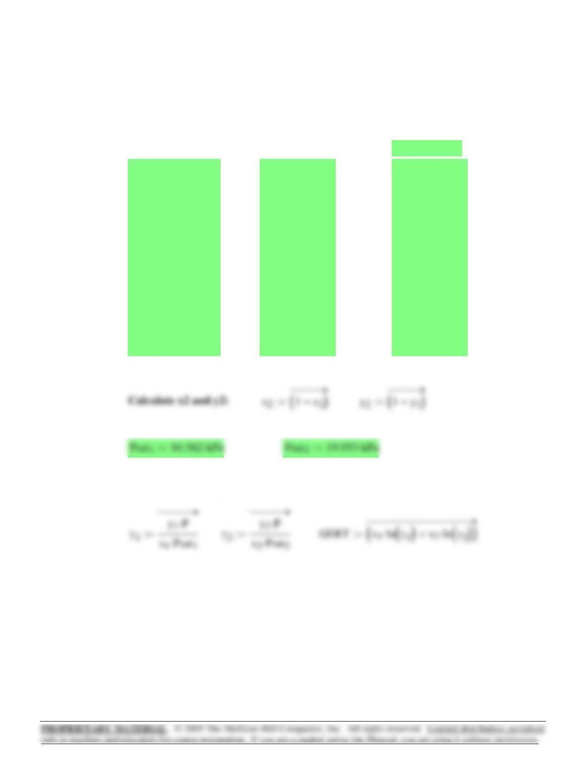
Calculate EXPERIMENTAL values of activity coefficients and
excess Gibbs energy.
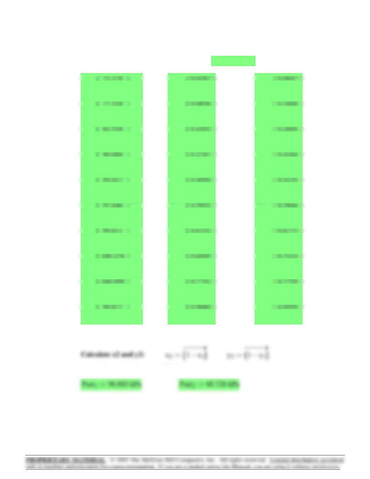
Vapor Pressures from equilibrium data:
i1n..:=n10=n rows P():=
Number of data points:
y1
0.5714
0.6268
0.6943
0.7345
0.7742
0.8085
0.8383
0.8733
0.8922
0.9141
⎛
⎜
⎜
⎜
⎜
⎜
⎜
⎜
⎜
⎜
⎜
⎜
⎜
⎜
⎝
⎞
⎟
⎟
⎟
⎟
⎟
⎟
⎟
⎟
⎟
⎟
⎟
⎠
:=
x1
0.1686
0.2167
0.3039
0.3681
0.4461
0.5282
0.6044
0.6804
0.7255
0.7776
⎛
⎜
⎜
⎜
⎜
⎜
⎜
⎜
⎜
⎜
⎜
⎜
⎜
⎜
⎝
⎞
⎟
⎟
⎟
⎟
⎟
⎟
⎟
⎟
⎟
⎟
⎟
⎠
:=
P
39.223
42.984
48.852
52.784
56.652
60.614
63.998
67.924
70.229
72.832
⎛
⎜
⎜
⎜
⎜
⎜
⎜
⎜
⎜
⎜
⎜
⎜
⎜
⎜
⎝
⎞
⎟
⎟
⎟
⎟
⎟
⎟
⎟
⎟
⎟
⎟
⎟
⎠
kPa⋅:=
T 333.15 K⋅:=
Methanol(1)/Water(2)– VLE data:12.1
Chapter 12 – Section A – Mathcad Solutions
374
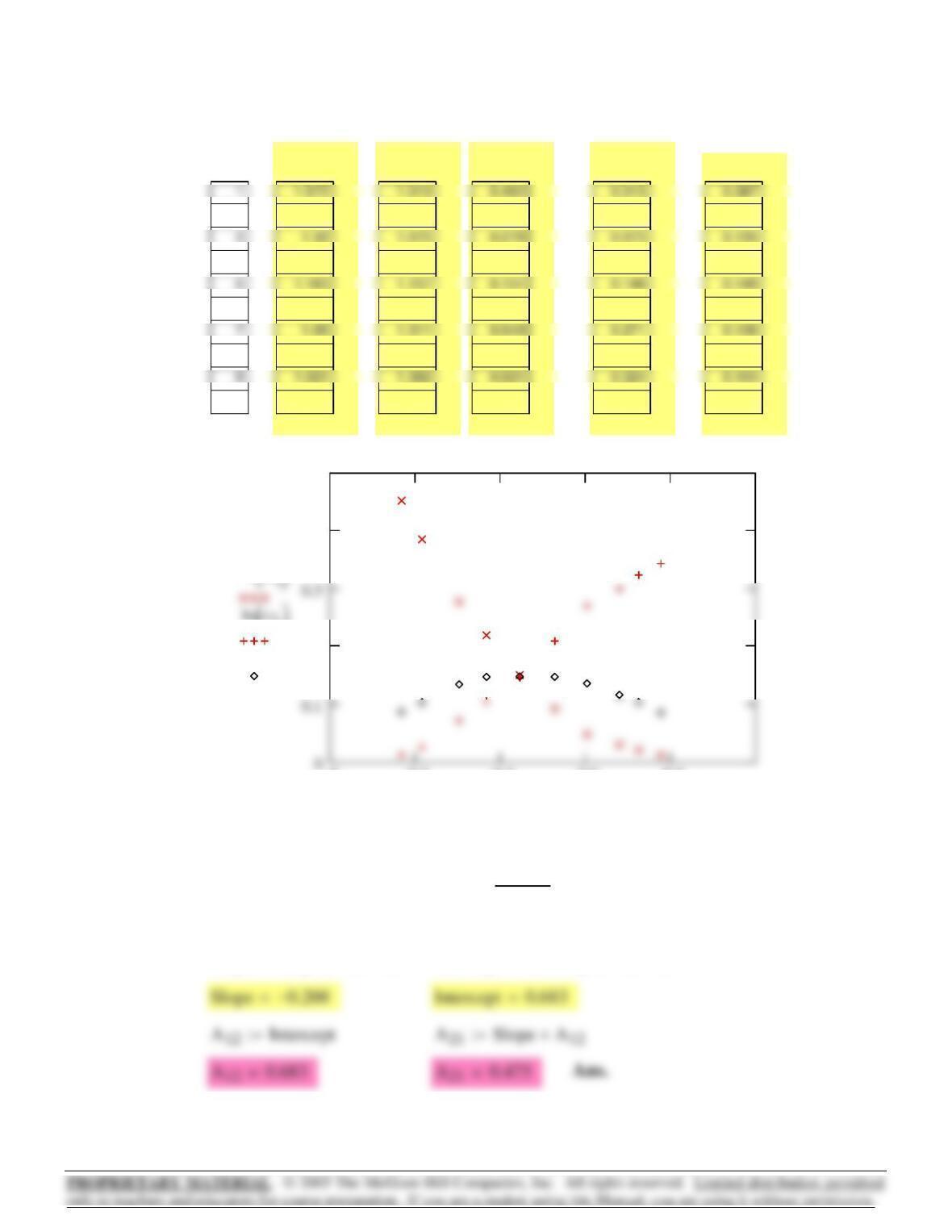
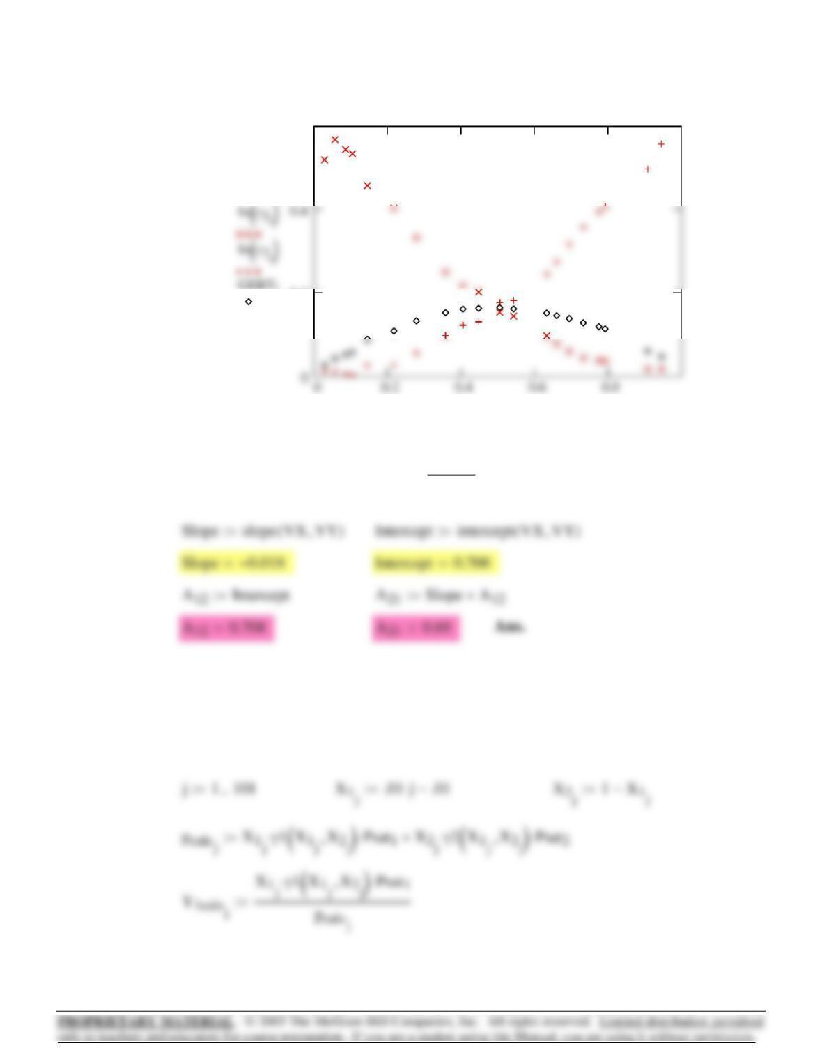
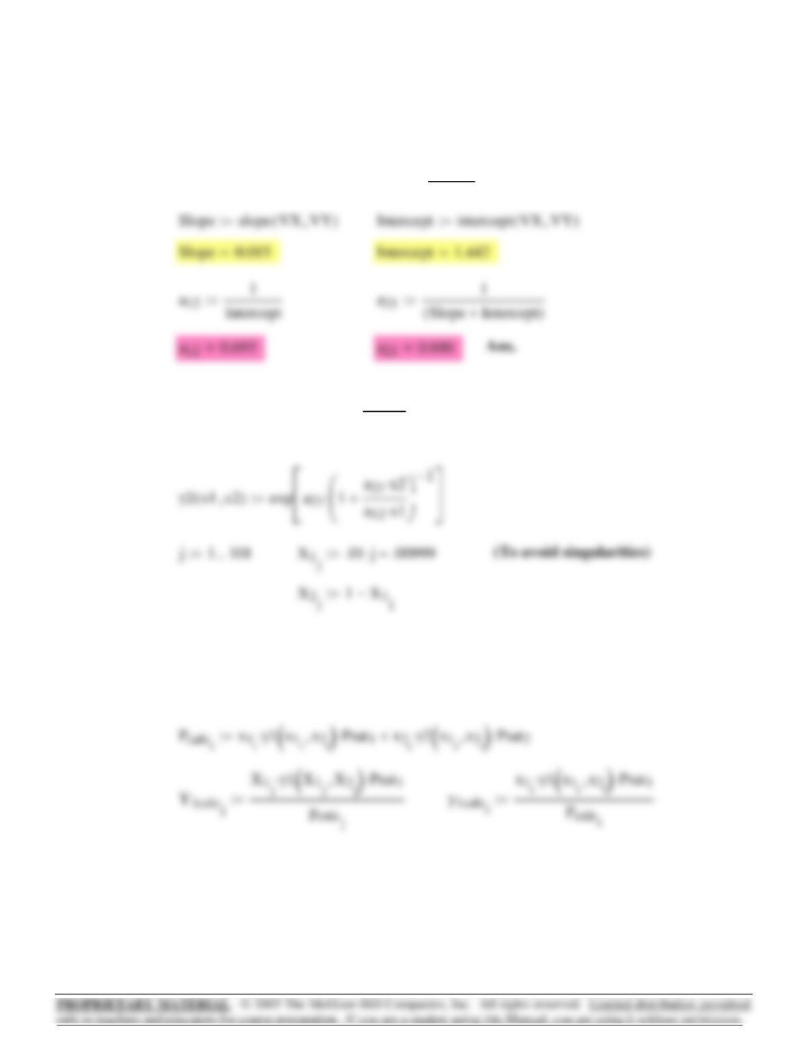
Intercept intercept VX VY,():=Slope slope VX VY,():=
VYi
GERTi
x1ix2i
⋅
:=VXix1i
:=
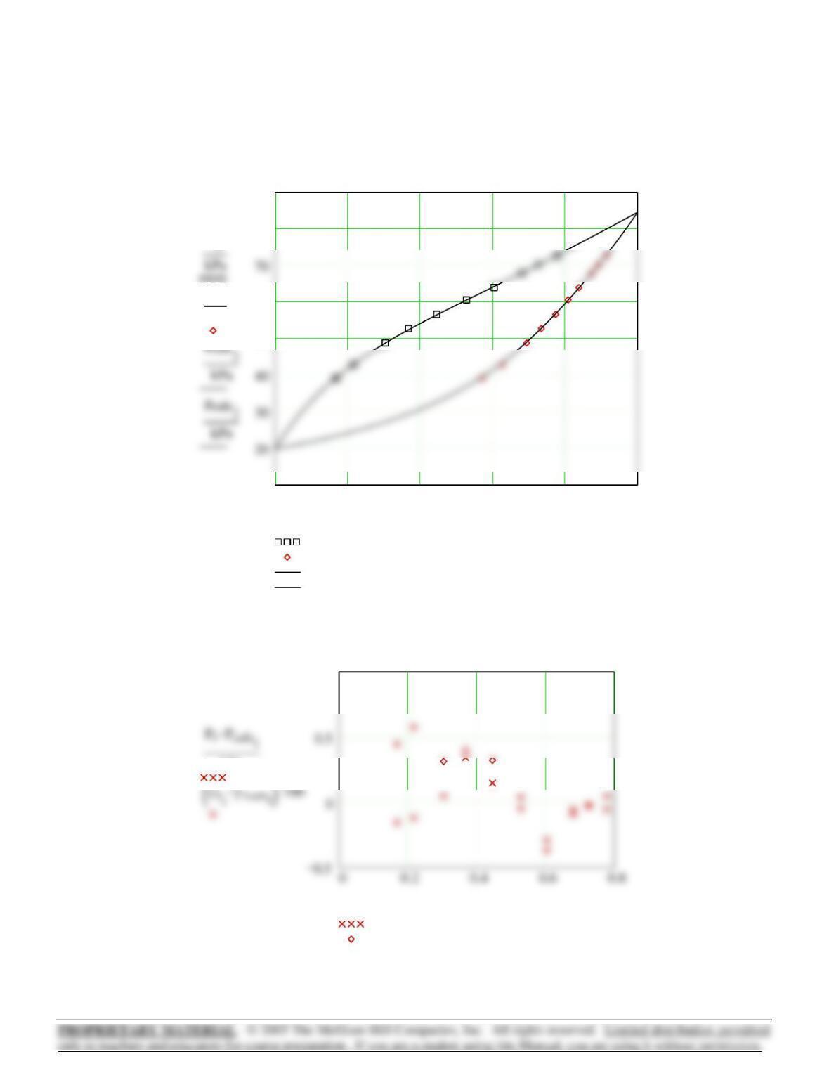
Fit GE/RT data to Margules eqn. by linear least squares:(a)
0 0.2 0.4 0.6 0.8
0.2
0.4
0.5
ln γ1i
()
GERTi
x1i
GERTi
0.104
0.148
0.148
0.117
0.086
=
i
2
4
6
8
10
=ln γ2i
(
)
0.026
0.106
0.209
0.3
0.343
=
ln γ1i
(
)
0.385
0.22
0.093
0.031
0.012
=
γ2i
1.026
1.112
1.233
1.35
1.41
=
γ1i
1.47
1.246
1.097
1.031
1.012
=
375
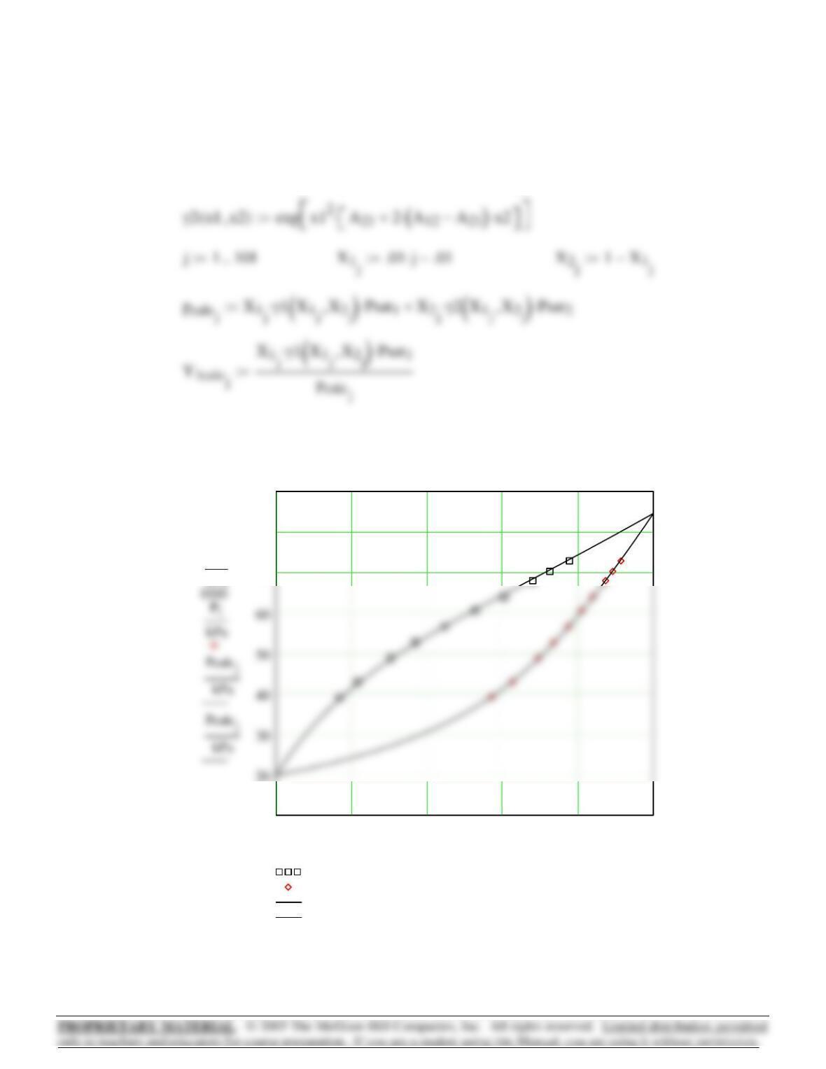
The following equations give CALCULATED values:
γ1x1x2,( ) exp x22A12 2A
21 A12
−
()
⋅x1⋅+
⎡
⎣
⎤
⎦
⋅
⎡
⎣
⎤
⎦
:=
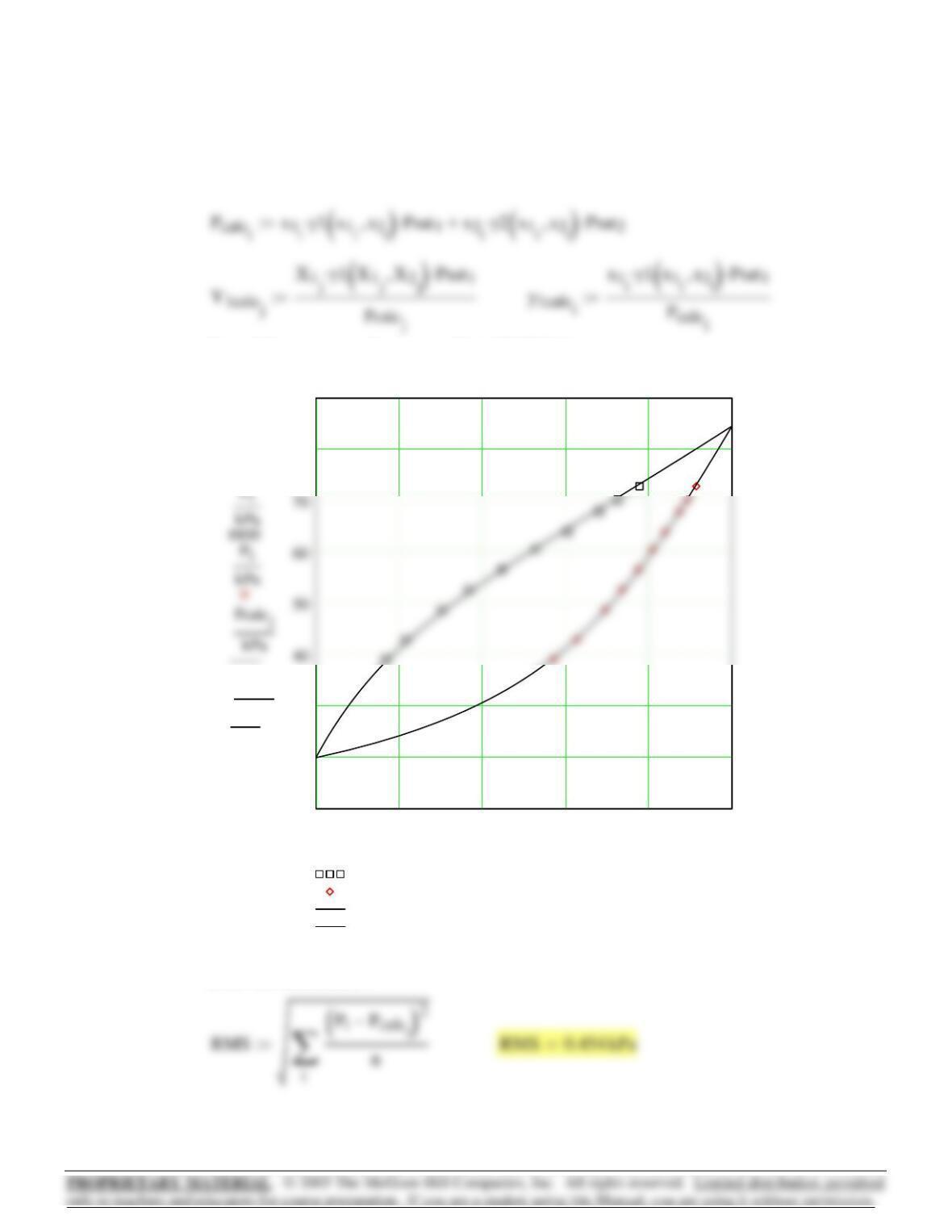
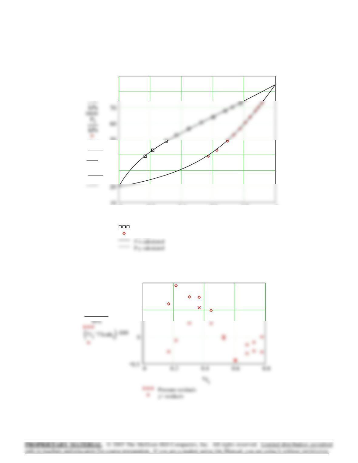
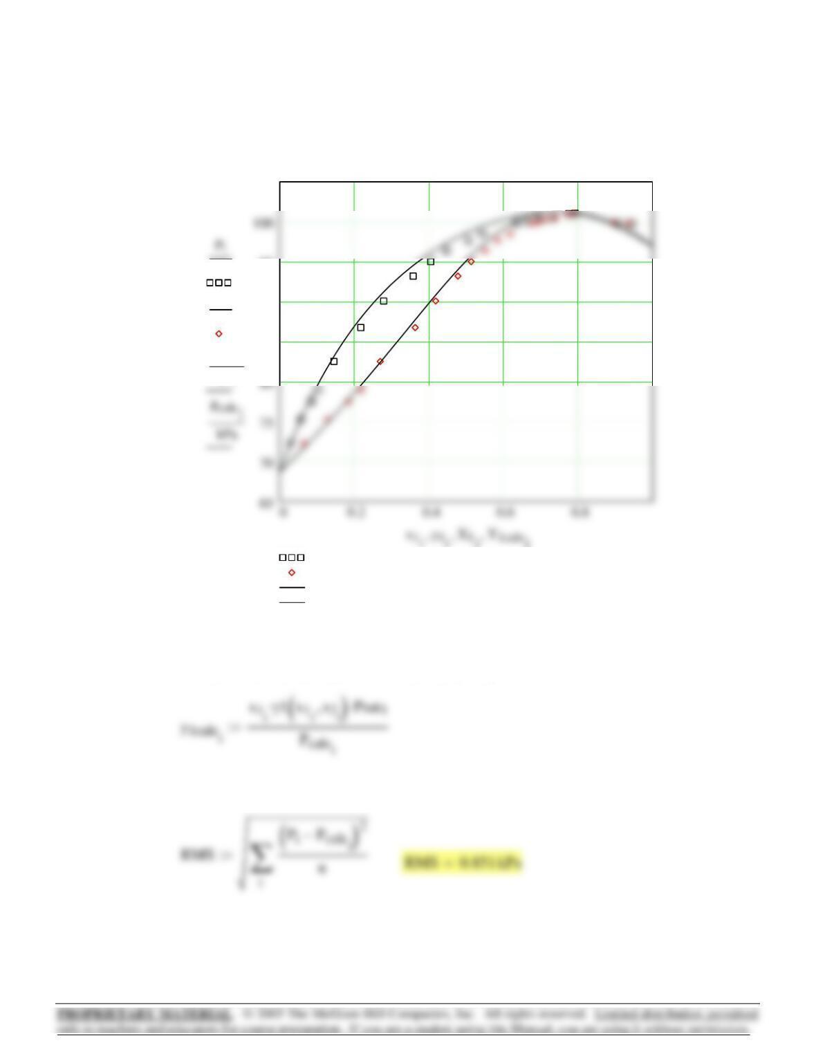
P-x,y Diagram: Margules eqn. fit to GE/RT data.
0 0.2 0.4 0.6 0.8
10
70
80
90
P-x data
P-y data
P-x calculated
P-y calculated
Pi
kPa
x1iy1i
,X1j
,Y1calcj
,
376
⎡
⎣
⎤
⎦
⎡
⎣
⎤
⎦
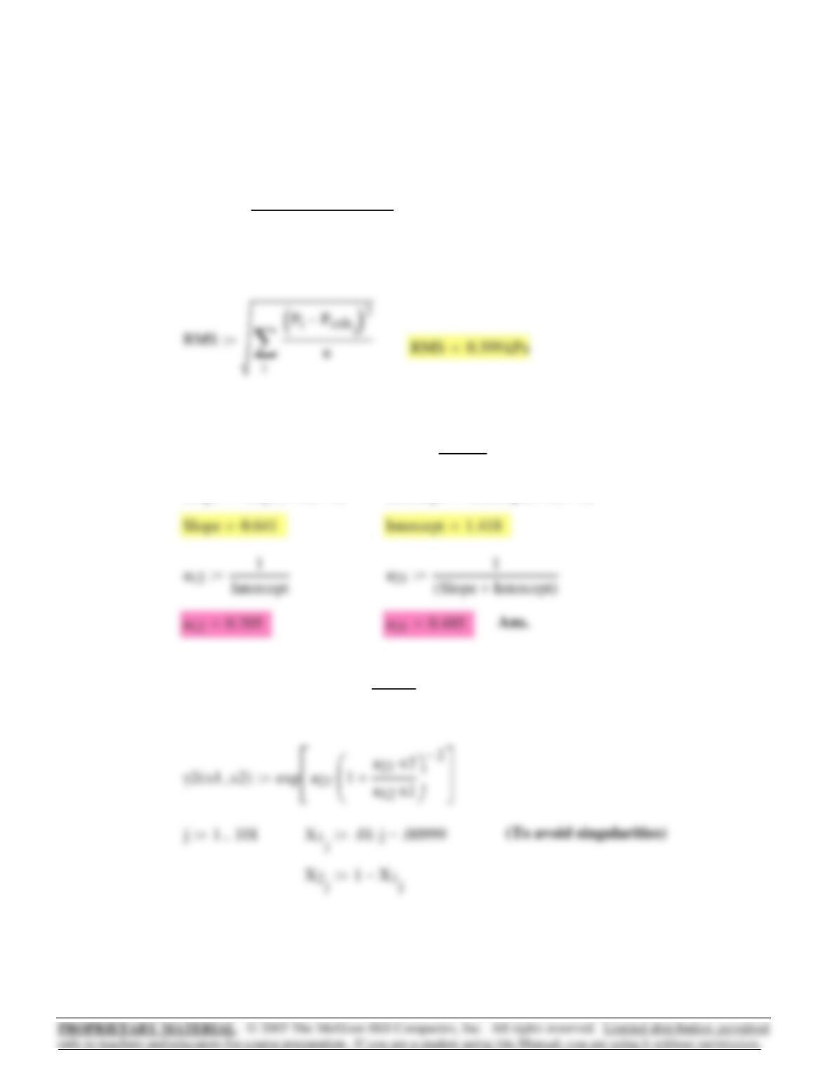
γ1x1x2,( ) exp a12 1a12 x1⋅
a21 x2⋅
+
⎛
⎜
⎝
⎞
⎠
2−
⋅
⎡
⎢
⎢
⎣
⎤
⎥
⎥
⎦
:=
Intercept intercept VX VY,():=Slope slope VX VY,():=
VYi
x1ix2i
⋅
GERTi
:=VXix1i
:=
Fit GE/RT data to van Laar eqn. by linear least squares:(b)
RMS deviation in P:
y1calci
x1iγ1x
1ix2i
,
()
⋅Psat1
⋅
Pcalci
:=
Pcalcix1iγ1x
1ix2i
,
()
⋅Psat1
⋅x2iγ2x
1ix2i
,
()
⋅Psat2
⋅+:=
377
⎜
⎢
⎢
⎥
⎥
pcalcjX1jγ1X
1jX2j
,
()
⋅Psat1
⋅X2jγ2X
1jX2j
,
()
⋅Psat2
⋅+:=
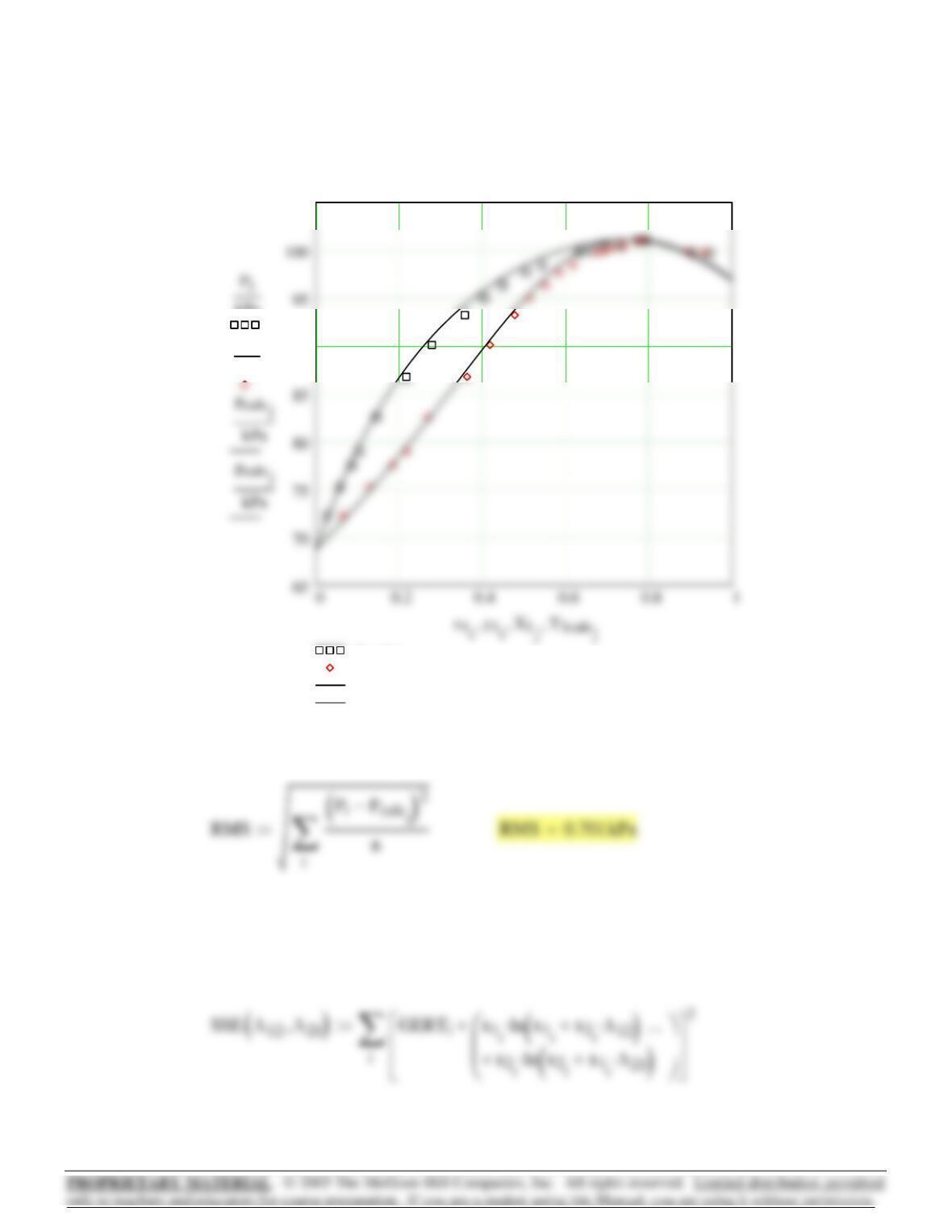
P-x,y Diagram: van Laar eqn. fit to GE/RT data.
0 0.2 0.4 0.6 0.8 1
10
20
30
80
90
P-x data
P-y data
P-x calculated
P-y calculated
pcalcj
kPa
x1iy1i
,X1j
,Y1calcj
,
RMS deviation in P:
378
γ1x1x2,()
exp x2
Λ12
x1 x2 Λ12
⋅+
Λ21
x2 x1 Λ21
⋅+
−
⎛
⎜
⎝
⎞
⎠
⋅
⎡
⎢
⎣
⎤
⎥
⎦
x1 x2 Λ12
⋅+
()
:=
⎜
⎜
SSE Λ12 Λ21
,
()
i
GERTix1iln x1ix2iΛ12
⋅+
()
⋅
x2iln x2ix1iΛ21
⋅+
()
⋅+
…
⎛
⎜
⎜
⎝
⎞
⎠
+
⎡
⎢
⎢
⎣
⎤
⎥
⎥
⎦
2
∑
:=
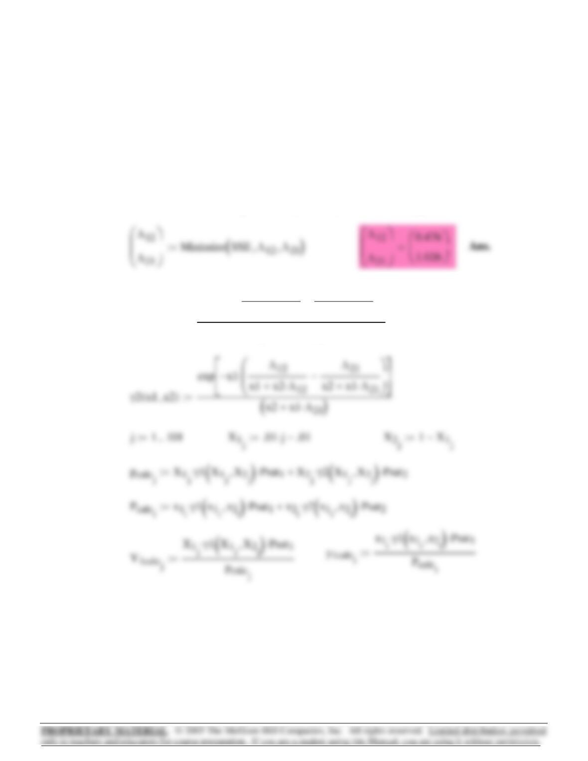
Λ21 1.0:=Λ12 0.5:=
Guesses:
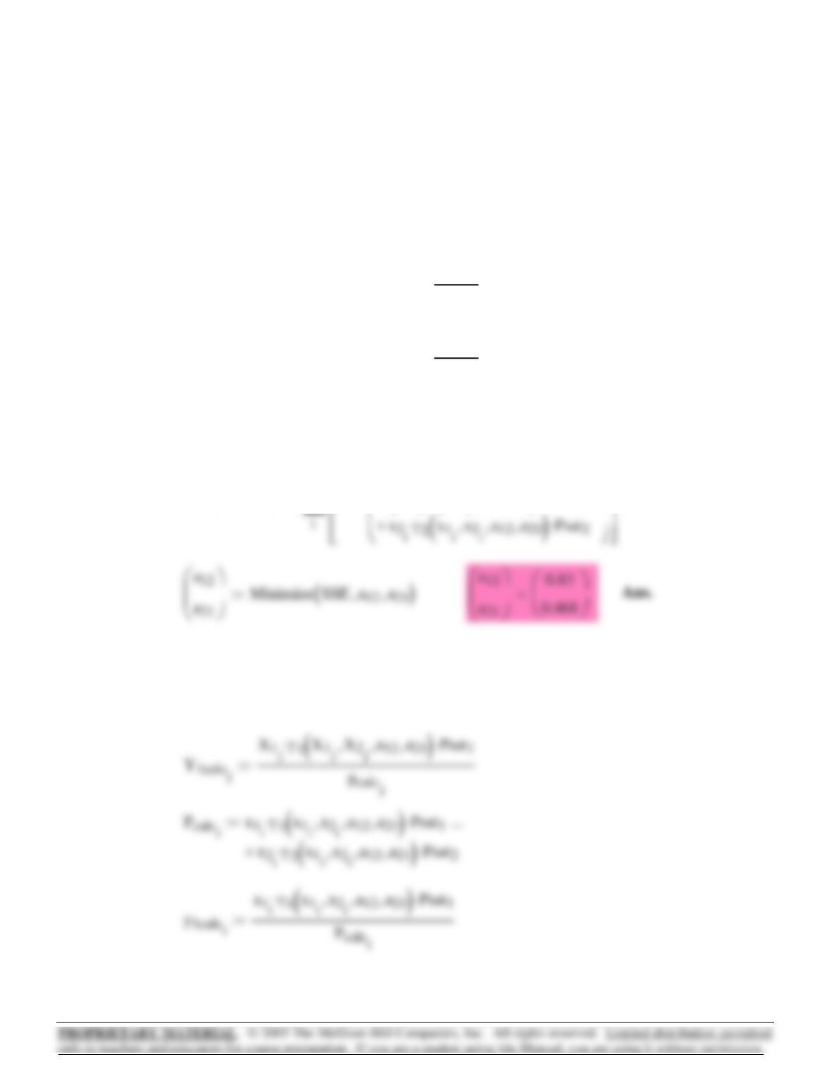
Minimize the sum of the squared errors using the Mathcad Minimize function.
Fit GE/RT data to Wilson eqn. by non-linear least squares.(c)
379
⎜
⎢
⎥
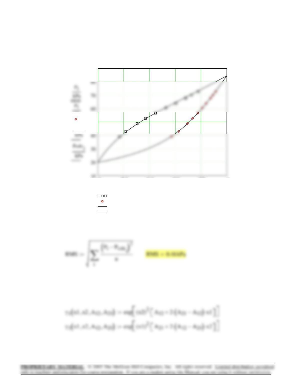
P-x,y diagram: Wilson eqn. fit to GE/RT data.
0 0.2 0.4 0.6 0.8 1
50
90
P-x data
P-y data
P-x calculated
P-y calculated
kPa
pcalcj
x1iy1i
,X1j
,Y1calcj
,
RMS deviation in P:
(d) BARKER’S METHOD by non-linear least squares.
Margules equation.
Guesses for parameters: answers to Part (a).
380
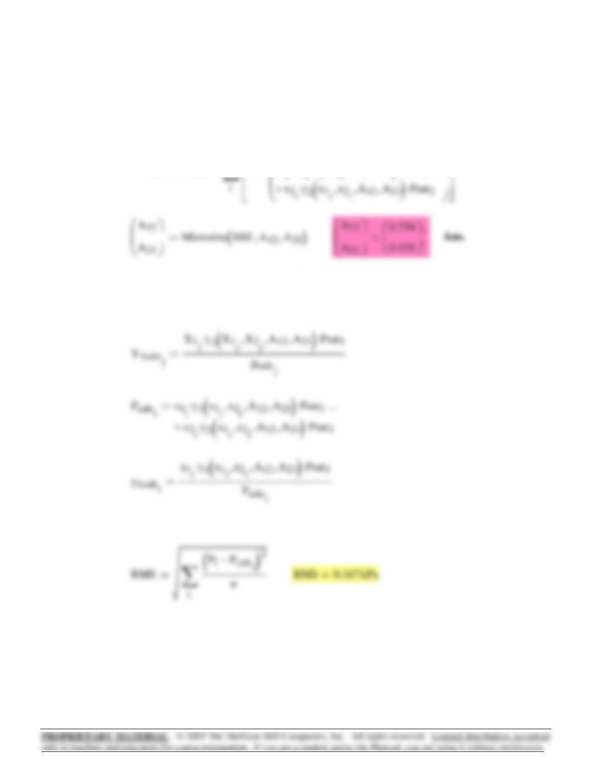
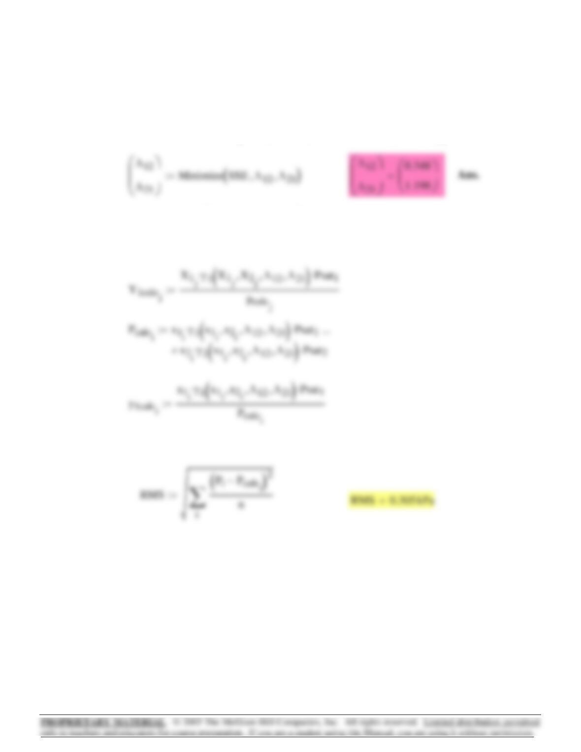
RMS deviation in P:
pcalcjX1jγ1X1jX2j
,A12
,A21
,
()
⋅Psat1
⋅
X2jγ2X1jX2j
,A12
,A21
,
()
⋅Psat2
⋅+
…:=
SSE A12 A21
,
()
Pix1iγ1x1ix2i
,A12
,A21
,
()
⋅Psat1
⋅
…
⎛
⎞
−
⎡
⎤
2
:=
A21 1.0:=A12 0.5:=
Guesses:
Minimize the sum of the squared errors using the Mathcad Minimize function.
381
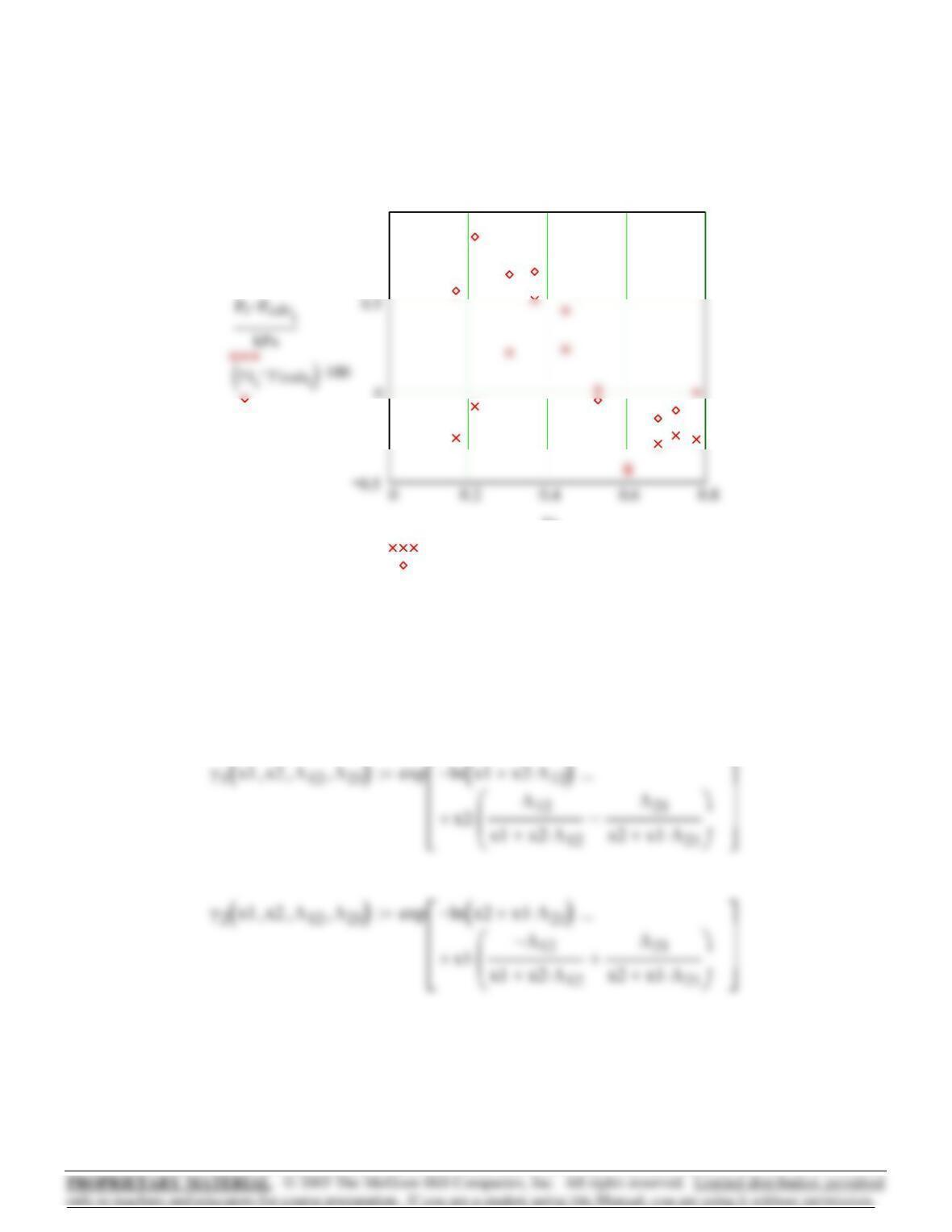
P-x-y diagram, Margules eqn. by Barker’s method
0 0.2 0.4 0.6 0.8 1
10
50
60
80
90
P-x data
P-y data
P-x calculated
P-y calculated
Pi
Pi
kPa
pcalcj
x1iy1i
,X1j
,Y1calcj
,
Residuals in P and y1
1
Pressure residuals
y1 residuals
kPa
x1i
382
pcalcjX1jγ1X1jX2j
,a12
,a21
,
()
⋅Psat1
⋅
X2jγ2X1jX2j
,a12
,a21
,
()
⋅Psat2
⋅+
…:=
SSE a12 a21
,
()
Pix1iγ1x1ix2i
,a12
,a21
,
()
⋅Psat1
⋅
…
⎛
⎜
⎞
−
⎡
⎢
⎤
⎥
2
∑
:=
a21 1.0:=a12 0.5:=
Guesses:
Minimize the sum of the squared errors using the Mathcad Minimize function.
γ2x1 x2,a12
,a21
,
()
exp a21 1a21 x2⋅
a12 x1⋅
+
⎛
⎜
⎝
⎞
⎠
2−
⋅
⎡
⎢
⎢
⎣
⎤
⎥
⎥
⎦
:=
γ1x1 x2,a12
,a21
,
()
exp a12 1a12 x1⋅
a21 x2⋅
+
⎛
⎜
⎝
⎞
⎠
2−
⋅
⎡
⎢
⎢
⎣
⎤
⎥
⎥
⎦
:=
j 1 101..:= X2j1X
1j
−:=X1j.01 j⋅.00999−:=
Guesses for parameters: answers to Part (b).
BARKER’S METHOD by non-linear least squares.
van Laar equation.
(e)
383

RMS deviation in P:
P-x,y diagram, van Laar Equation by Barker’s Method
0 0.2 0.4 0.6 0.8 1
10
20
30
50
60
80
90
P-x data
P-y data
kPa
Pi
kPa
pcalcj
x1iy1i
,X1j
,Y1calcj
,
384
Λ21 1.0:=Λ12 0.5:=
Guesses:
Minimize the sum of the squared errors using the Mathcad Minimize function.
X2j1X
1j
−:=X1j.01 j⋅.01−:=j 1 101..:=
Guesses for parameters: answers to Part (c).
Wilson equation.
BARKER’S METHOD by non-linear least squares.(f)
1
Pressure residuals
y1 residuals
x1i
Residuals in P and y1.
385
SSE Λ12 Λ21
,
()
i
Pix1iγ1x1ix2i
,Λ
12
,Λ
21
,
()
⋅Psat1
⋅
x2iγ2x1ix2i
,Λ
12
,Λ
21
,
()
⋅Psat2
⋅+
…
⎛
⎜
⎜
⎝
⎞
⎠
−
⎡
⎢
⎢
⎣
⎤
⎥
⎥
⎦
2
∑
:=
pcalcjX1jγ1X1jX2j
,Λ
12
,Λ
21
,
()
⋅Psat1
⋅
X2jγ2X1jX2j
,Λ
12
,Λ
21
,
()
⋅Psat2
⋅+
…:=
RMS deviation in P:
386
⎜
⎜
P-x,y diagram, Wilson Equation by Barker’s Method
0 0.2 0.4 0.6 0.8 1
30
40
50
80
90
P-x data
P-y data
Pi
pcalcj
kPa
pcalcj
kPa
x1iy1i
,X1j
,Y1calcj
,
Residuals in P and y1.
0.5
1
PiPcalci
−
387
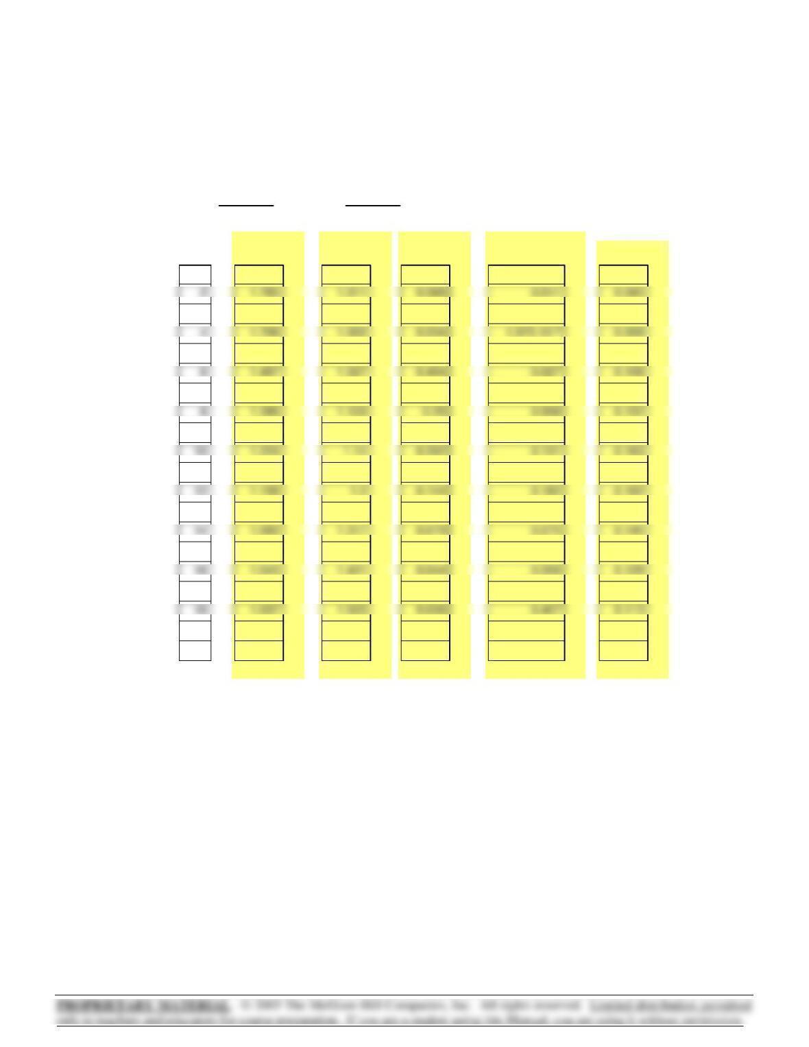
Vapor Pressures from equilibrium data:
i1n..:=n20=n rows P():=
Number of data points:
y1
0.1295
0.2190
0.3633
0.4779
0.5512
0.6174
0.6926
0.7383
0.7876
0.9336
⎛
⎜
⎜
⎜
⎜
⎜
⎜
⎜
⎜
⎜
⎜
⎜
⎜
⎜
⎜
⎜
⎜
⎜
⎜
⎜
⎜
⎜
⎝
⎞
⎟
⎟
⎟
⎟
⎟
⎟
⎟
⎟
⎟
⎟
⎟
⎟
⎟
⎟
⎟
⎟
⎟
⎟
⎟
⎟
⎠
:=x1
0.0570
0.1046
0.2173
0.3579
0.4480
0.5432
0.6605
0.7327
0.7922
0.9448
⎛
⎜
⎜
⎜
⎜
⎜
⎜
⎜
⎜
⎜
⎜
⎜
⎜
⎜
⎜
⎜
⎜
⎜
⎜
⎜
⎜
⎜
⎝
⎞
⎟
⎟
⎟
⎟
⎟
⎟
⎟
⎟
⎟
⎟
⎟
⎟
⎟
⎟
⎟
⎟
⎟
⎟
⎟
⎟
⎠
:=P
75.279
78.951
86.762
93.206
96.365
98.462
99.950
100.467
101.059
99.799
⎛
⎜
⎜
⎜
⎜
⎜
⎜
⎜
⎜
⎜
⎜
⎜
⎜
⎜
⎜
⎜
⎜
⎜
⎜
⎜
⎜
⎜
⎝
⎞
⎟
⎟
⎟
⎟
⎟
⎟
⎟
⎟
⎟
⎟
⎟
⎟
⎟
⎟
⎟
⎟
⎟
⎟
⎟
⎟
⎠
kPa⋅:=
T 328.15 K⋅:=
Acetone(1)/Methanol(2)– VLE data:12.3
388
Calculate EXPERIMENTAL values of activity coefficients and
excess Gibbs energy.
γ1
y1P⋅
x1Psat1
⋅
→
⎯
⎯
⎯
:= γ2
y2P⋅
x2Psat2
⋅
→
⎯
⎯
⎯
:= GERT x1ln γ1
()
⋅x2ln γ2
()
⋅+
()
→
⎯
⎯⎯⎯⎯⎯⎯⎯
⎯
:=
γ1i
1.682
1.723
1.58
1.396
1.243
1.166
1.102
1.062
1.039
1.017
1.018
=γ2i
1.013
1.006
1.026
1.057
1.13
1.193
1.278
1.374
1.485
1.644
1.747
=ln γ1i
()
0.52
0.544
0.458
0.334
0.218
0.153
0.097
0.06
0.039
0.017
0.018
=ln γ2i
()
0.013
-3
5.815·10
0.026
0.055
0.123
0.177
0.245
0.317
0.395
0.497
0.558
=
i
1
3
5
7
9
11
13
15
17
19
20
=GERTi
0.027
0.052
0.089
0.133
0.161
0.165
0.151
0.139
0.119
0.061
0.048
=
389
γ2x1x2,( ) exp x12A21 2A
12 A21
−
()
⋅x2⋅+
⎡
⎣
⎤
⎦
⋅
⎡
⎣
⎤
⎦
:=
γ1x1x2,( ) exp x22A12 2A
21 A12
−
()
⋅x1⋅+
⎡
⎣
⎤
⎦
⋅
⎡
⎣
⎤
⎦
:=
The following equations give CALCULATED values:
VYi
GERTi
x1ix2i
⋅
:=VXix1i
:=
Fit GE/RT data to Margules eqn. by linear least squares:(a)
0.2
0.6
x1i
390
P-x,y Diagram: Margules eqn. fit to GE/RT data.
85
90
95
105
P-x data
P-y data
P-x calculated
P-y calculated
kPa
Pi
kPa
pcalcj
kPa
Pcalcix1iγ1x
1ix2i
,
()
⋅Psat1
⋅x2iγ2x
1ix2i
,
()
⋅Psat2
⋅+:=
RMS deviation in P:
391
pcalcjX1jγ1X
1jX2j
,
()
⋅Psat1
⋅X2jγ2X
1jX2j
,
()
⋅Psat2
⋅+:=
⎜
⎢
⎢
⎥
⎥
γ1x1x2,( ) exp a12 1a12 x1⋅
a21 x2⋅
+
⎛
⎜
⎝
⎞
⎠
2−
⋅
⎡
⎢
⎢
⎣
⎤
⎥
⎥
⎦
:=
VYi
x1ix2i
⋅
GERTi
:=VXix1i
:=
Fit GE/RT data to van Laar eqn. by linear least squares:(b)
392
P-x,y Diagram: van Laar eqn. fit to GE/RT data.
90
105
P-x data
P-y data
P-x calculated
P-y calculated
kPa
Pi
kPa
RMS deviation in P:
(c) Fit GE/RT data to Wilson eqn. by non-linear least squares.
Minimize the sum of the squared errors using the Mathcad Minimize function.
Guesses: Λ12 0.5:= Λ21 1.0:=
393