An Introduction to Shear Strength Chapter 12
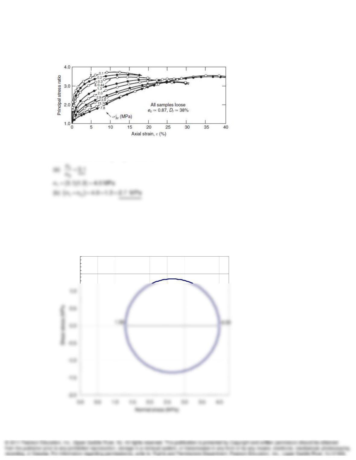
12-17. For the data shown in Fig. 12.5(a), what is (a) the principal stress difference and (b) the
principal stress ratio at an axial strain of 12% for an effective confining pressure of 1.3 MPa?
SOLUTION:
c3
Given : 12% and 1.3 MPa
12-18. For the conditions given in Problem 12.17, plot the Mohr circle.
SOLUTION:
C 2.65, R 1.35
1.5
2.0
An Introduction to Shear Strength Chapter 12
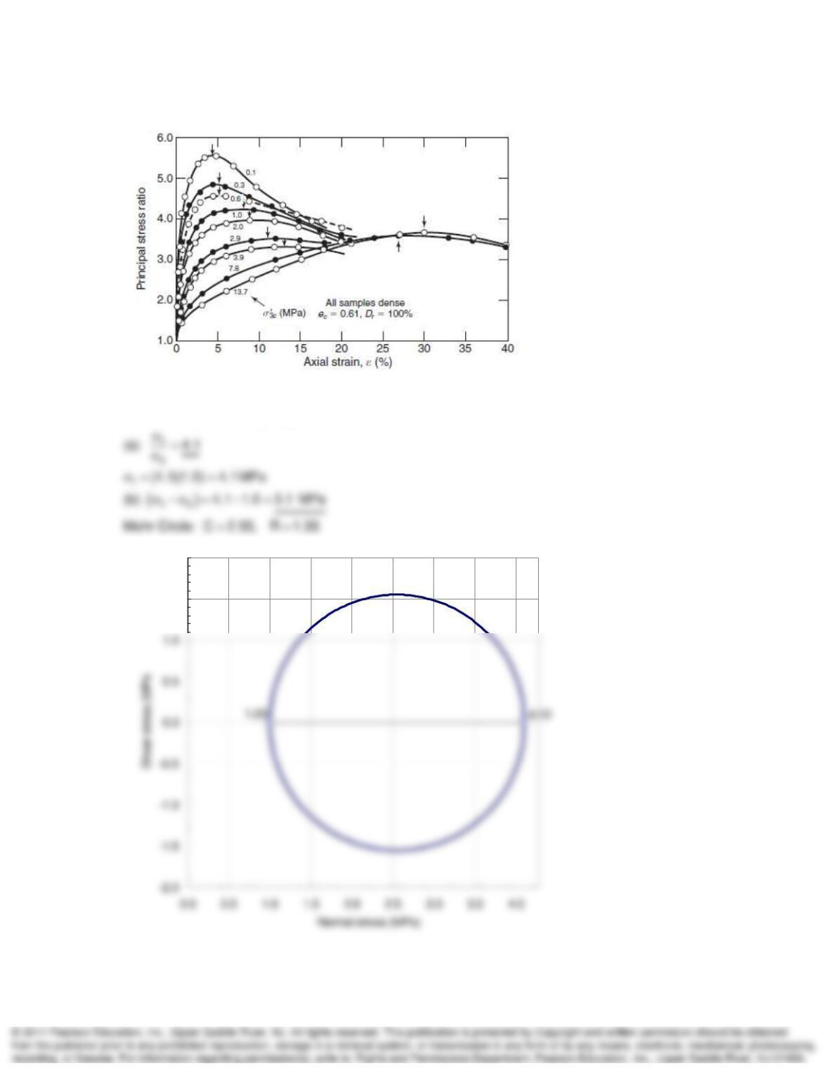
12-19. Do Problems 12.17 and 12.18 for the data shown in Fig. 12.6(a). Use
c = 1.0 MPa.
SOLUTION:
c3
Given : 12% and 1.0 MPa
1.5
2.0
An Introduction to Shear Strength Chapter 12
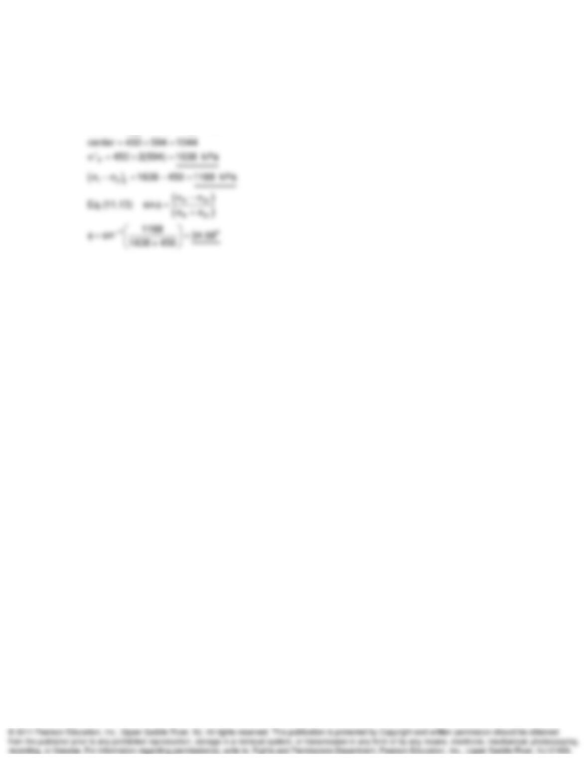
12-22. A drained triaxial test is performed on a sand with
’3c=
’3f = 450 kPa. At failure,
max =
594 kPa. Find
’1f, (
1 –
3)f,, and
’.
SOLUTION:
max 3f
radius 594, ‘ 450
An Introduction to Shear Strength Chapter 12
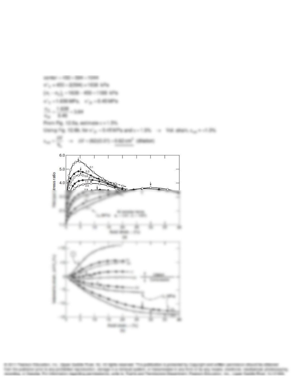
12-23. Assume the sand of Problem 12.22 is Sacramento River sand at a void ratio of 0.6. If the
initial volume of the specimen was 62 cm3, what change in volume would you expect during
shear?
SOLUTION:
max 3f
radius 594, ‘ 450
An Introduction to Shear Strength Chapter 12
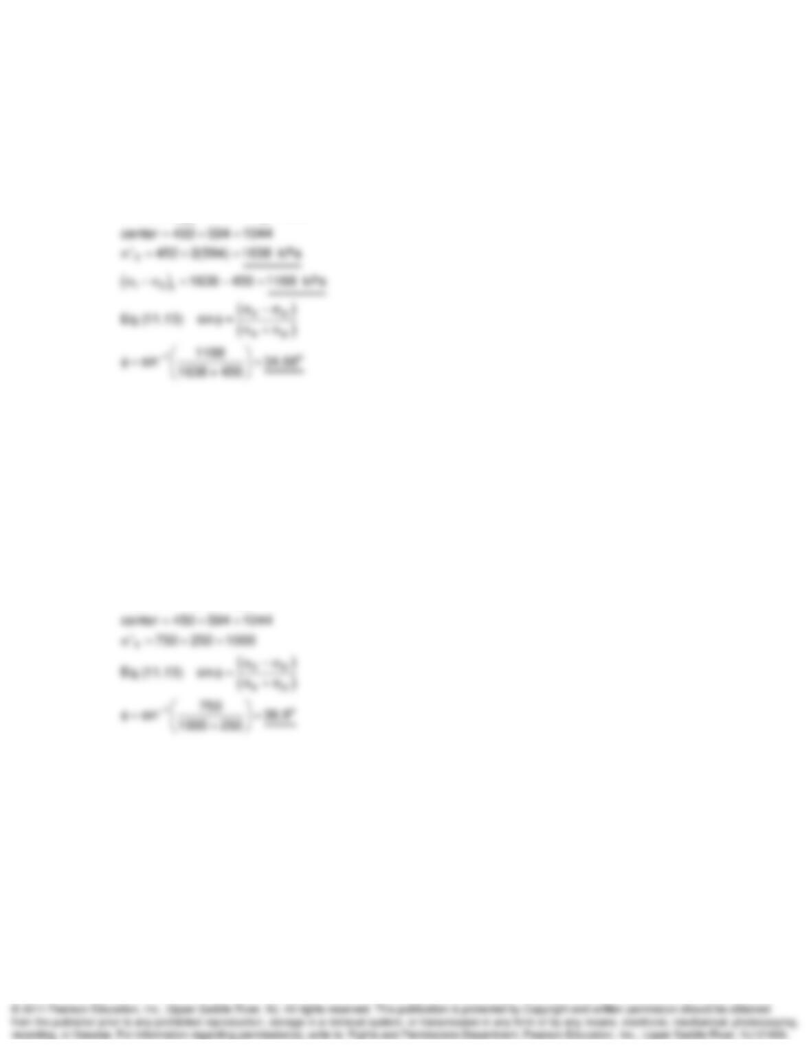
12-24. A silty sand is tested consolidated-drained in a triaxial cell where both principal stresses
at the start of the test were 625 kPa. If the total axial stress at failure is 2.04 MPa while the
horizontal pressure remains constant, compute the angle of shearing resistance and the
theoretical orientation of the failure plane with respect to the horizontal.
SOLUTION:
max 3f
radius 594, ‘ 450
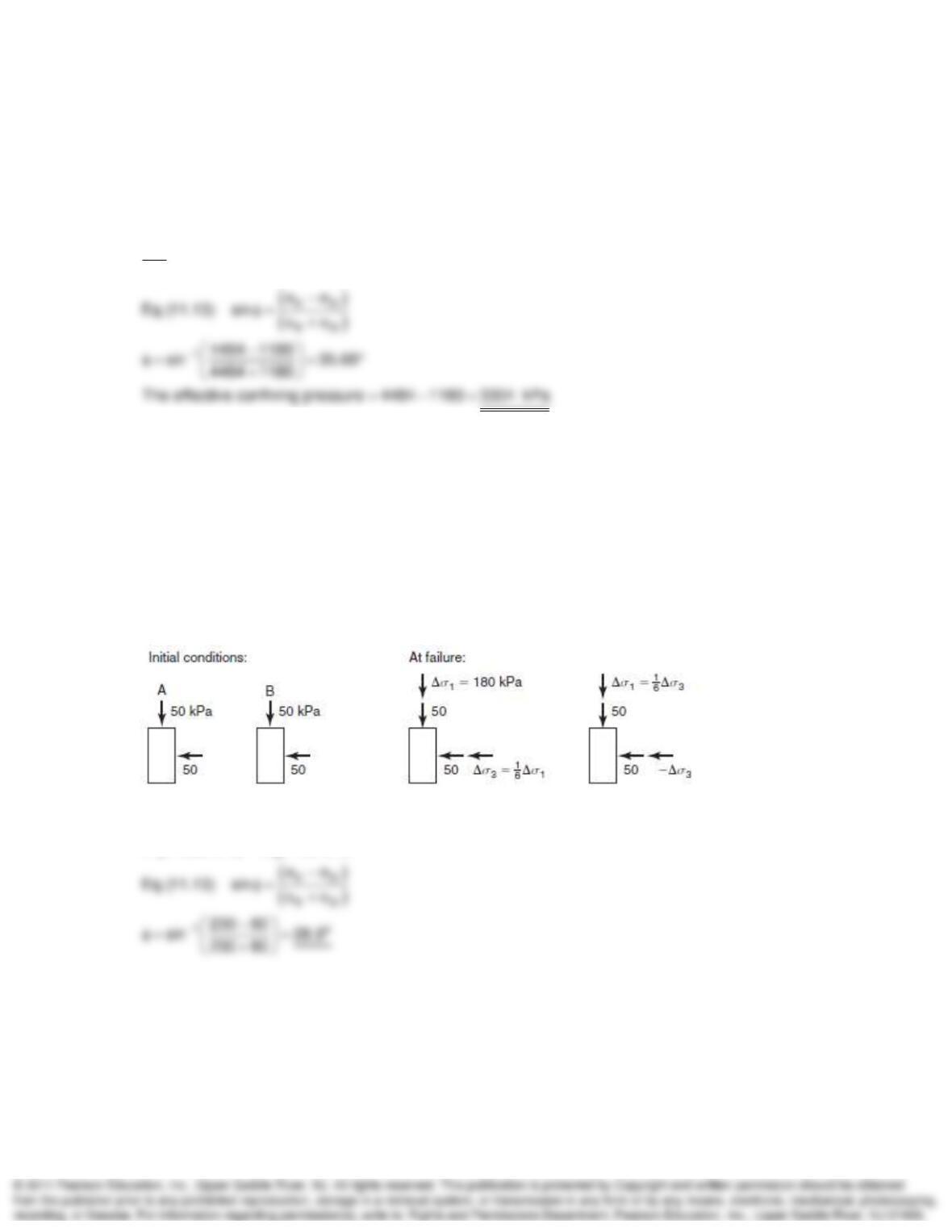
12-25. A specimen of sand failed when (
1 –
3) was 750 kPa. If the hydrostatic consolidation
stress was 250 kPa, compute the angle of shearing resistance of the sand. What else can you
say about the sand?
SOLUTION:
3f 1 3 f
‘ 250, 750
An Introduction to Shear Strength Chapter 12
12-26. A specimen of sand at the field density is known to have a (
1/
3)max of 3.8. If such a
specimen is hydrostatically consolidated to 1180 kPa in a triaxial test apparatus, at what effective
confining pressure will the specimen fail if the vertical stress is held constant? (This is a lateral
extension test.)
SOLUTION:
1f 3f 1f
3f
3.8, ‘ 1180 (1180)(3.8) 4484
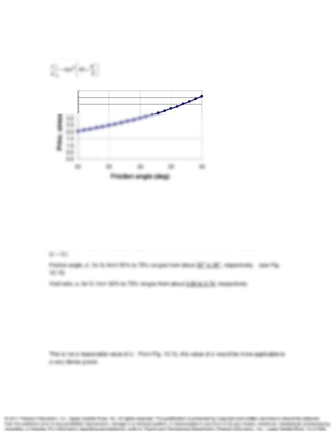
12-27. Two CD triaxial tests are conducted on identical specimens of the same sand. Both
specimens are initially consolidated hydrostatically to 50 kPa; then each specimen is loaded as
shown. Specimen A failed when the applied
1 was 180 kPa. Make the necessary calculations
to (a) plot the Mohr circles at failure for both tests, and (b) determine
’ for the sand.
SOLUTION:
1f 3 f
‘230kPa,‘ 80kPa
An Introduction to Shear Strength Chapter 12
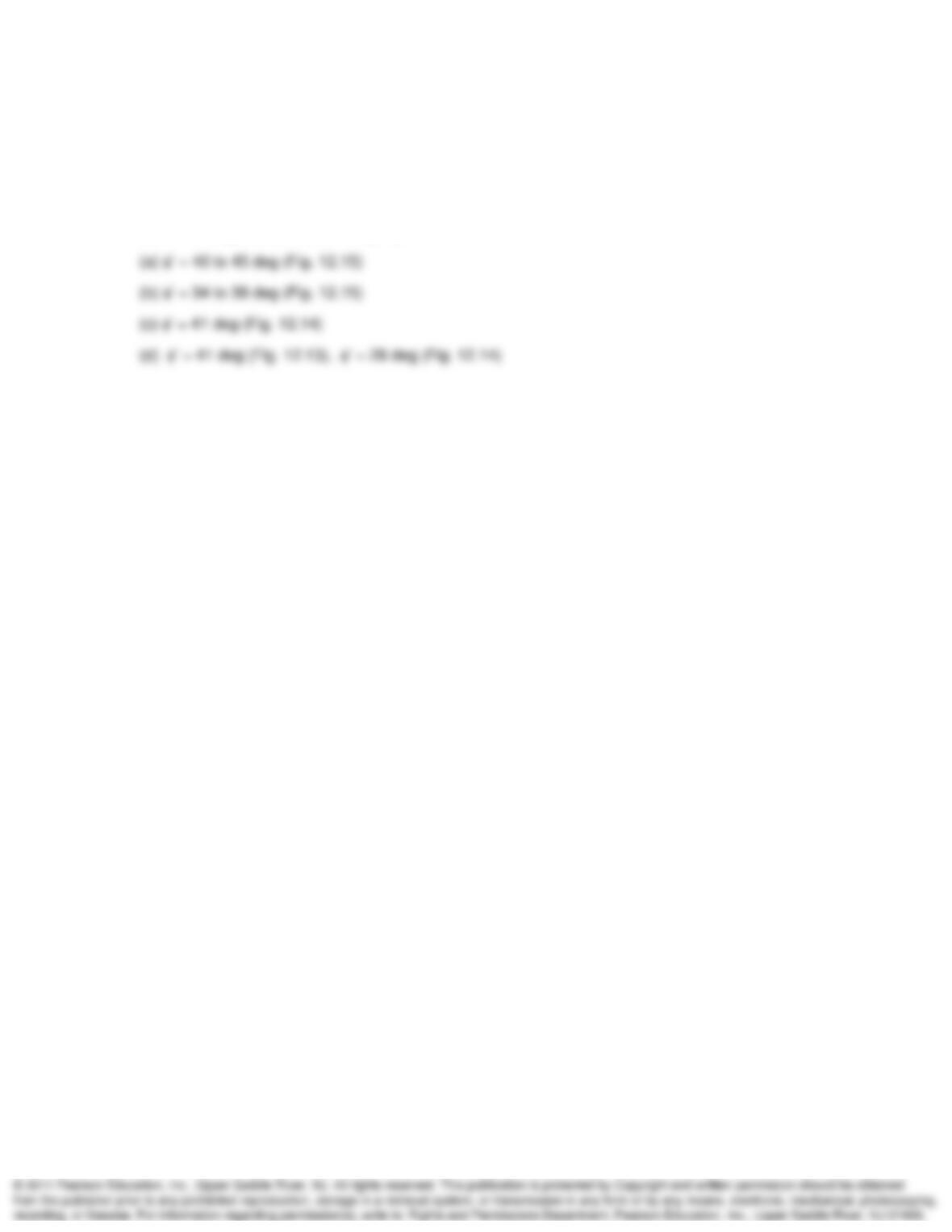
12-28. Plot a graph of
’1/
’3 versus
’.
SOLUTION:
3.5
4.0
4.5
5.0
o
12-29. Estimate the shear strength parameters of a fine (beach) sand (SP). Estimate the
minimum and maximum void ratios.
SOLUTION:
’ depends on relative density among a number of other items as described in Section 12.5.
12-30. A subrounded to subangular sand has a D10 of about 0.1 mm and a uniformity coefficient
of 3. The angle of shearing resistance measured in the direct shear test was 47°. Is this
reasonable? Why or why not?
SOLUTION:
An Introduction to Shear Strength Chapter 12
12-31. Estimate the
’ values for (a) a well-graded sandy gravel (GW) at a density of 1.9 Mg/m3;
(b) a poorly graded silty sand with a field density of 1.70 Mg/m3; (c) an SW material at 100%
relative density; and (d) a poorly graded gravel with an in situ void ratio of 0.5.
SOLUTION:
Estimate ranges of ’ values using Fig. 12.15.
An Introduction to Shear Strength Chapter 12
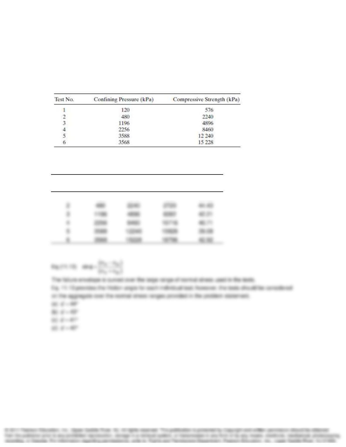
12-32. The results of a series of CD triaxial tests on a medium dense, cohesionless sand are
summarized in the table below. The void ratios for all the test specimens were approximately the
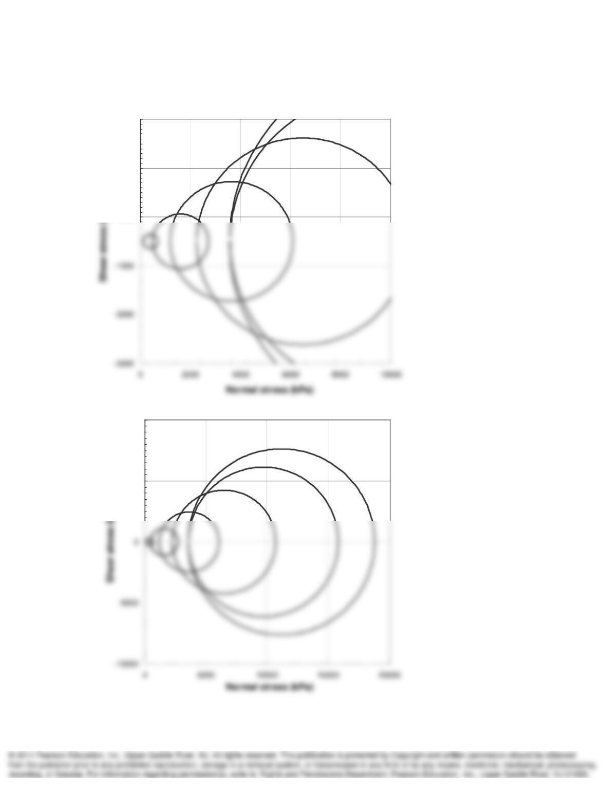
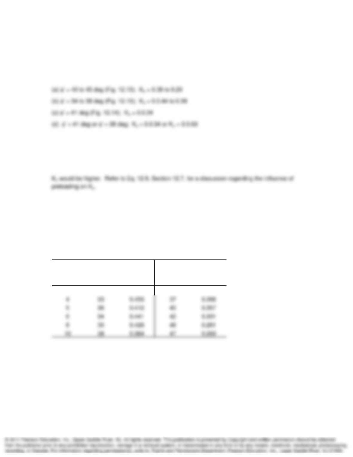
same at the start of the test. Plot the strength circles and draw the Mohr failure envelope for this
series of tests. What angle of internal friction should be used in solving stability problems in which
the range of normal stresses is (a) 0–500 kPa; (b) 1000–1500 kPa; (c) 3–6 MPa; and (d) 0–6
MPa?
SOLUTION:
Test No.
3
1
–
3
1
‘
(kPa) (kPa) (kPa) (deg)
1 120 576 696 44.90
Mohr circles shown on the next page.
An Introduction to Shear Strength Chapter 12
12-32 continued.
1000
3000
5000
)
5000
10000
)
An Introduction to Shear Strength Chapter 12
12-33. Estimate the values of the coefficient of earth pressure at rest, Ko, for the four soils of
Problem 12-31.
SOLUTION:
o
(Eq. 12.8) K 1 sin ‘
12-34. If the sands of Problem 12.33 had been preloaded, would your estimate of be any
different? If so, would it be higher or lower? Why?
SOLUTION:
12-35. Estimate Ko for sands 1, 4, 5, 6, 8, and 10 in Table 12.1 for relative densities of 40% and
85%.
SOLUTION:
o
(Eq. 12.8) K 1 sin ‘
Sand No. ‘K
o
‘K
o
(deg) (deg)
1 28 0.531 35 0.426
(Loose, D
r
= 40%) (Dense, D
r
= 85%)
An Introduction to Shear Strength Chapter 12
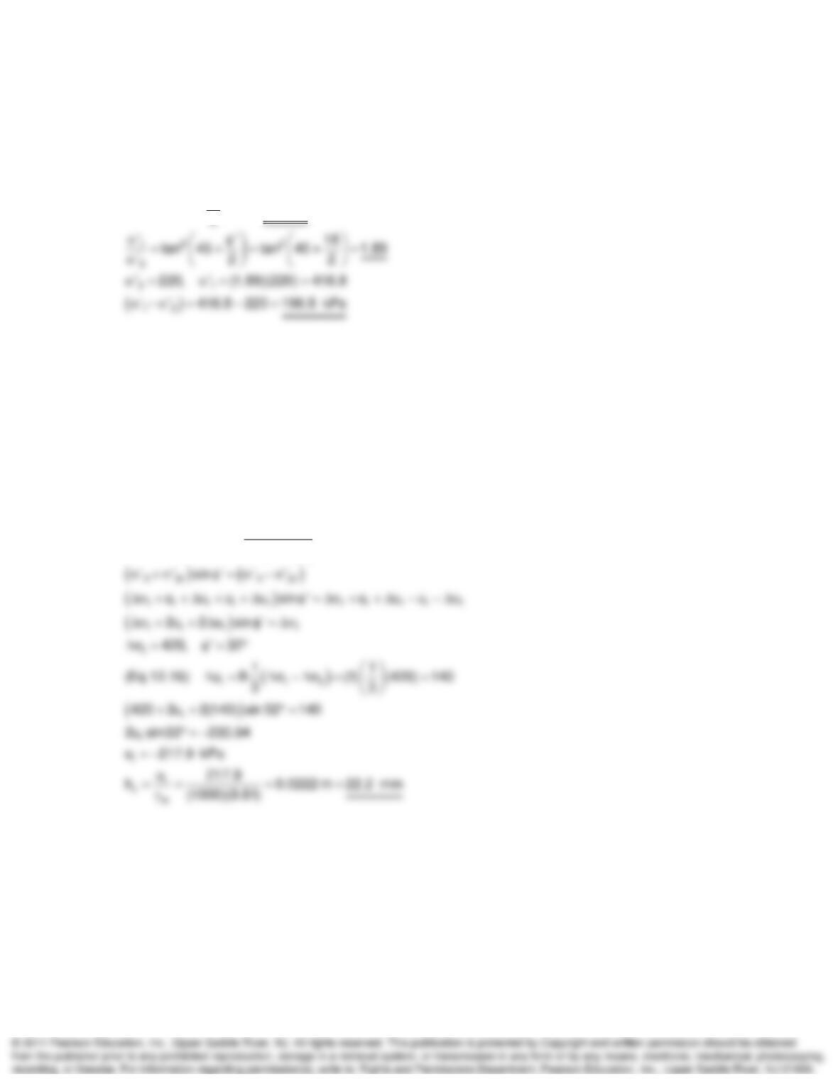
12-38. A CD axial compression triaxial test on a normally consolidated clay failed along a clearly
defined failure plane of 54°. The cell pressure during the test was 220 kPa. Estimate
’, the
maximum principal stress ratio and the principal stress difference at failure.
SOLUTION:
‘
54 45 ‘ 18
12-39. An unconfined compression test is performed on a dense silt. Previous drained triaxial
tests on similar samples of the silt gave
’ = 32o. If the unconfined compressive strength was 420
kPa, estimate the height of capillary rise in this soil above the ground water table. (Hint: Find the
effective confining pressure acting on the specimen. Draw elements similar to Fig. 12.40.)
SOLUTION:
1f 3 f
1f 3 f
1f 3 f
‘230kPa,‘ 80kPa
”
Eq. (11.13) sin ”
An Introduction to Shear Strength Chapter 12
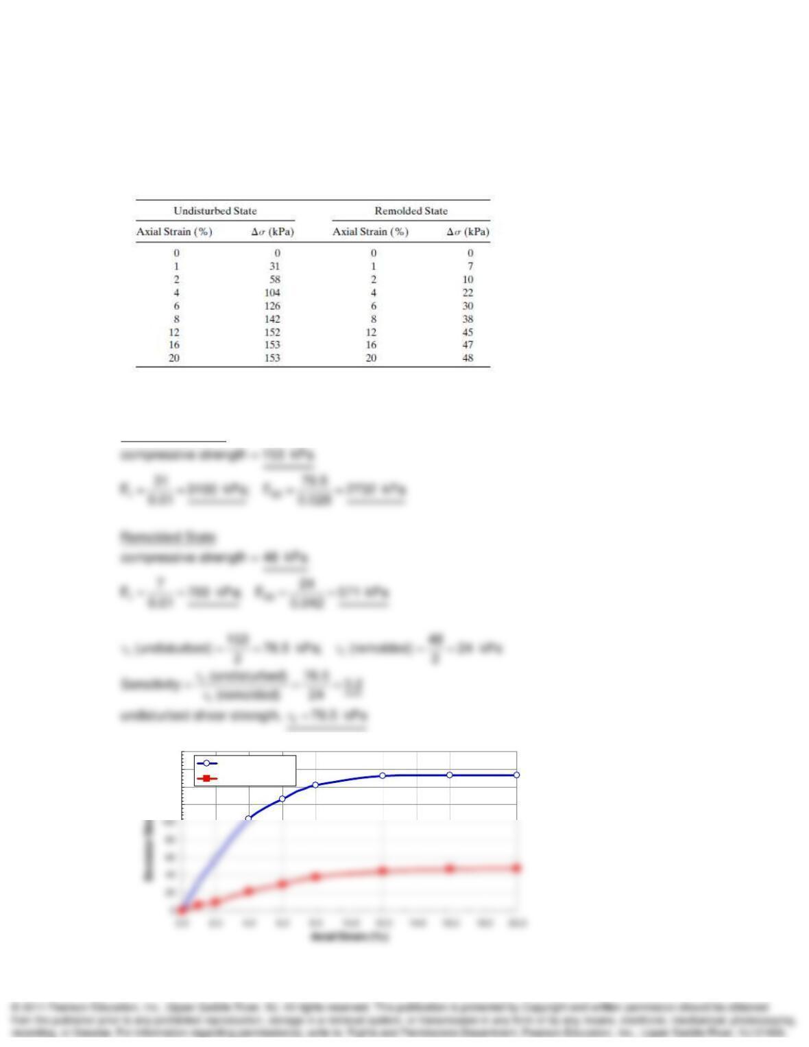
12-43. The results of unconfined compression tests on a sample of clay in both the undisturbed
and remolded states are summarized below. Determine the compressive strength, the initial
tangent modulus of deformation, and the secant modulus of deformation at 50% of the
compressive strength for both the undisturbed and remolded specimens. Determine the
sensitivity of the clay. What shear strength would you use?
SOLUTION:
Solutions obtained from the stress-strain plot shown below.
Undisturbed State
120
140
160
180
undisturbed state
remolded state
An Introduction to Shear Strength Chapter 12
12-45. For the data shown in Fig. 8.5, estimate the unconfined compressive strength and the
sensitivity of this soil. Typical values for the clay are LL = 88, PL = 43, and PI = 45.
SOLUTION: