This file contains the exercises, hints, and solutions for Chapter 10 of the
book ”Introduction to the Design and Analysis of Algorithms,” 3rd edition, by
Exercises 10.1
1. Consider the following version of the post office location problem: (Prob-
2. Solve the following linear programming problems geometrically.
(a)
maximize 3+
subject to −+≤1
3. Consider the linear programming problem
minimize 1+2
subject to +≥4
4. Would the solution to problem (10.2) be different if its inequality con-
straints were strict, i.e., +4and +36respectively?
5. Trace the simplex method on
6. Trace the simplex method on the problem of Example 1 in Section 6.6
7. Determine how many iterations the simplex method needs to solve the
problem
not.
9. BProve that no linear programming problem can have exactly ≥1
optimal solutions unless =1
10. If a linear programming problem
maximize P
=1
subject to P
=1 ≤for =12
1
2 ≥0
2
Hints to Exercises 10.1
2. Sketch the feasible region of the problem in question. Follow this up by
3. Sketch the feasible region of the problem. Then choose values of the pa-
rameters 1and 2to obtain a desired behavior of the objective function’s
level lines.
5. Trace the simplex method on the instances given, as was done for an
example in the text.
6. When solving the problem by hand, you might want to start by getting rid
of fractional coefficients in the problem’s statement. Also, note that the
7. The specifics of the problem make it possible to see the optimal solution
8. Consider separately two versions of the problem: continuous and 0-1 (see
Example 2 in Section 6.6).
10. a. You will need to use the notion of a matrix transpose, defined as the
matrix whose rows are the columns of the given matrix.
b. Apply the general definition to the specificproblemgiven. Notethe
3
Solutions to Exercises 10.1
1. The problem is to find a value of that minimizes ()= 1
P
=1 |−|
which can be simplified to minimizing ()=P
=1 |−|since 1
is a con-
stant. Here is an iterative improvement algorithm that does this. Select
2. a. The feasible region of the linear programming problem
maximize 3+
subject to −+≤1
2+≤4
≥0≥0
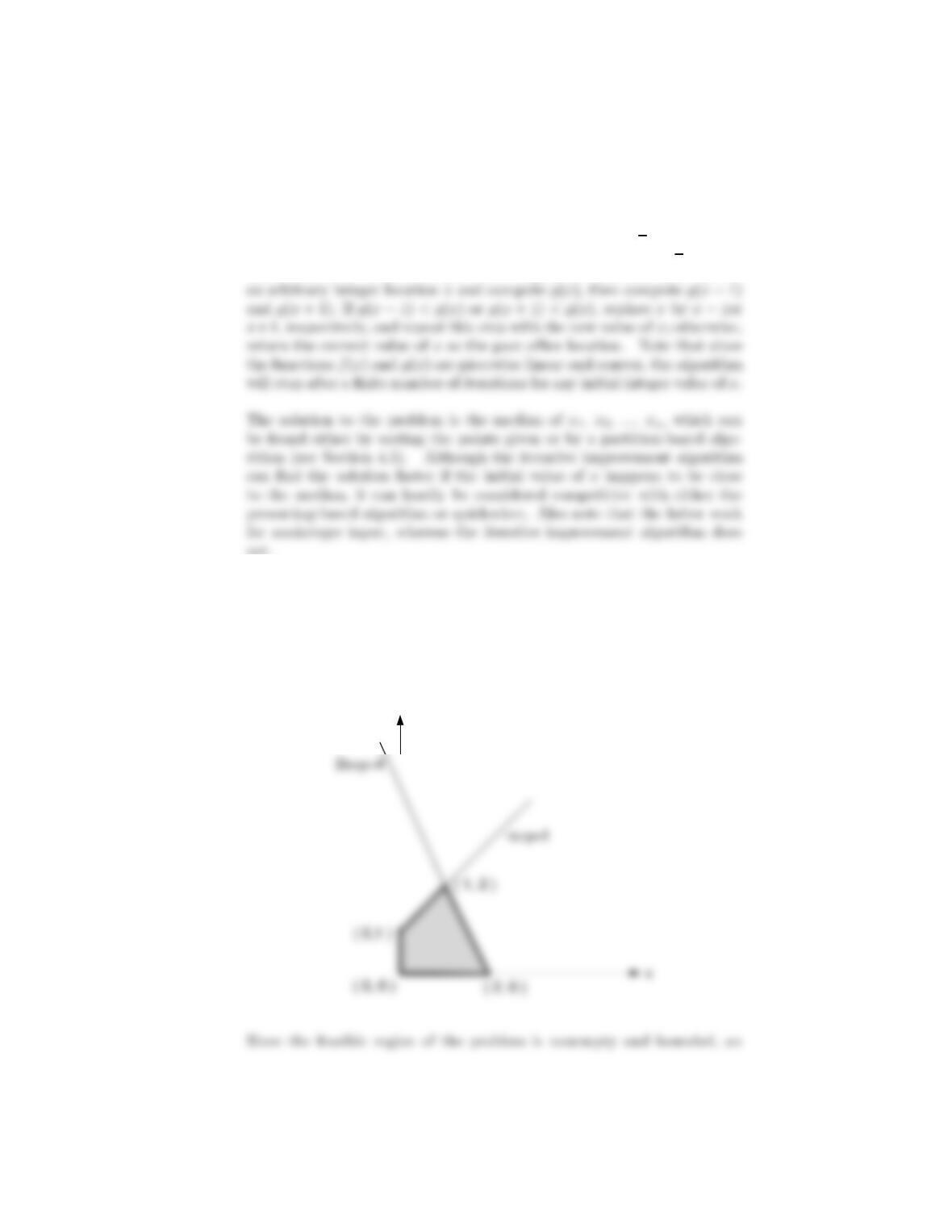
is given in the following figure:
y
4
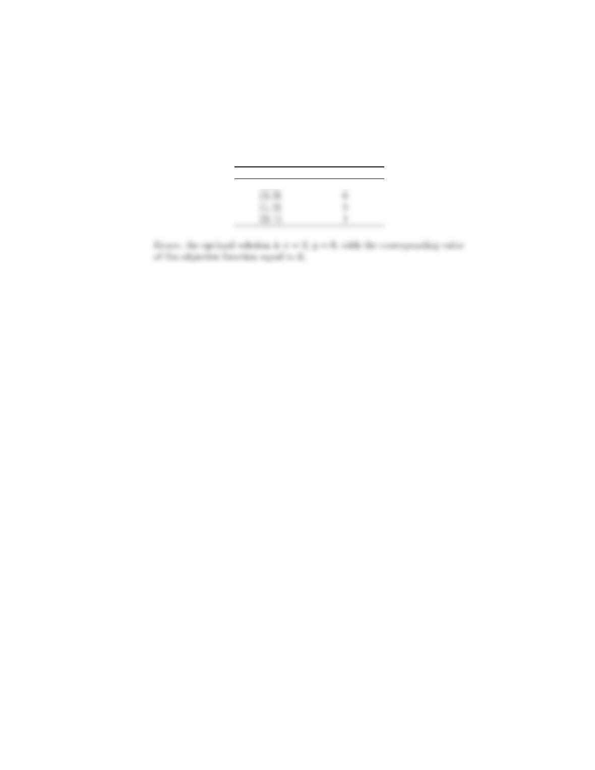
optimal solution exists and can be found at one of the extreme points of
the feasible region. The extreme points and the corresponding values of
the objective function are given in the following table:
Extreme point Value of 3+
(00) 0
5
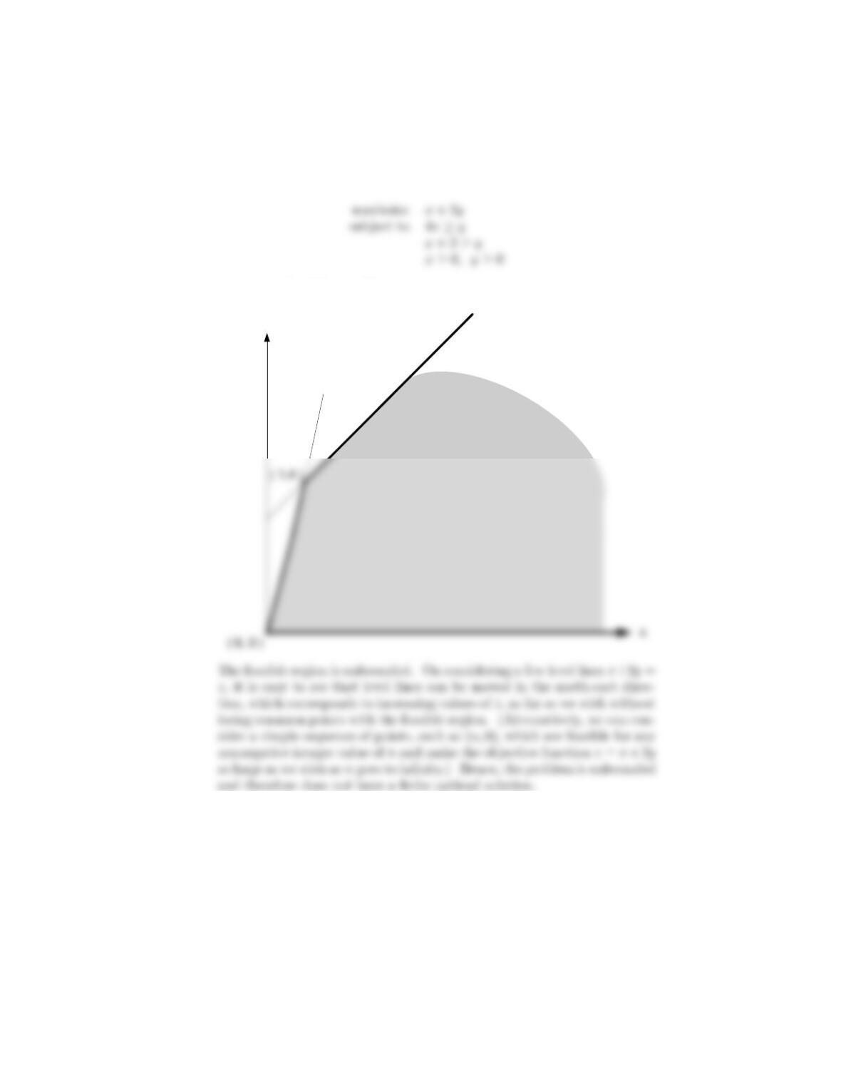
b. The feasible region of the linear programming problem
is given in the following figure:
y
y=4x
y=x+3
6
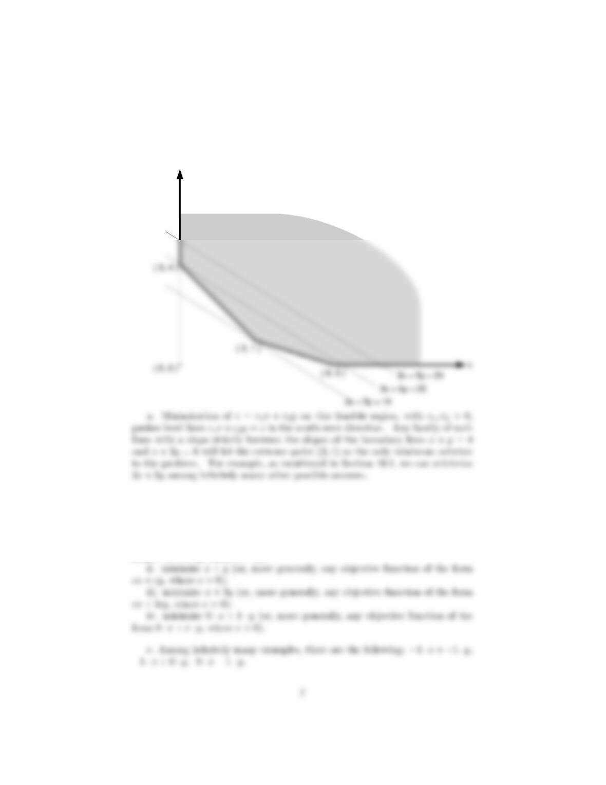
3. The feasible region of the problem with the constraints +≥4
+3≥6≥0≥0is given in Figure 10.3 of Section 10.1:
y
b. For a linear programming problem to have infinitely many solutions, the
optimal level line of its objective function must contain a line segment that is
a part of the feasible region’s boundary. Hence, there are four qualitatively
distinct answers:
i. minimize 1·+0·(or, more generally, any objective function of the
form ·+0·,where0);
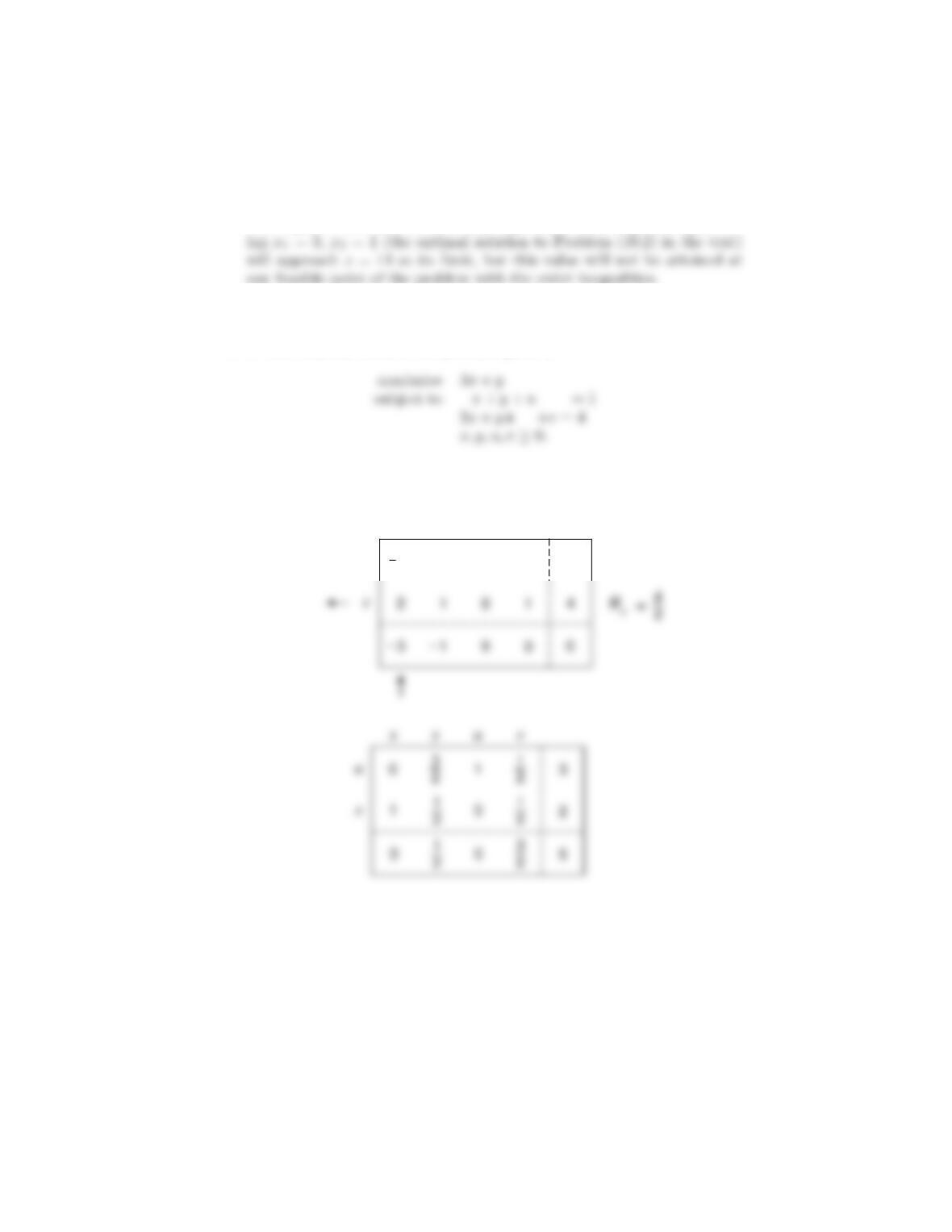
4. The problem with the strict inequalities does not have an optimal solution:
The objective function values of any sequence of feasible points approach-
5. a. The standard form of the problem given is
Here are the tableaux generated by the simplex method in solving this
problem:
11101
xyuv
u
The optimal solution found is =2=0with the maximal value of the
objective function equal to 6
8
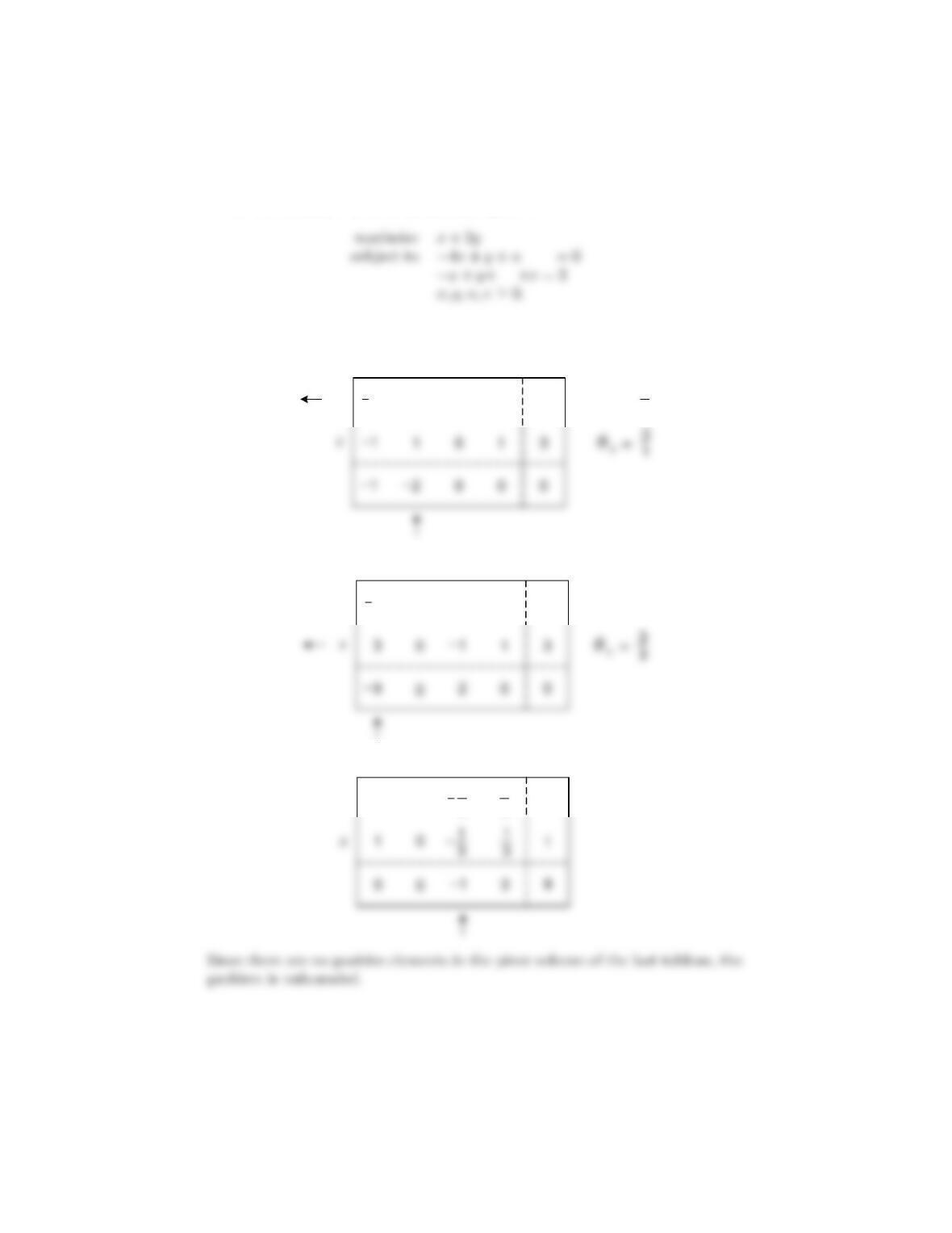
b. The standard form of the problem given is
Here are the tableaux generated by the simplex method in solving this problem:
41100
xyuv
u
~
0u = 0
1
41100
xyuv
y
014
34
xyuv
y
1
3
9
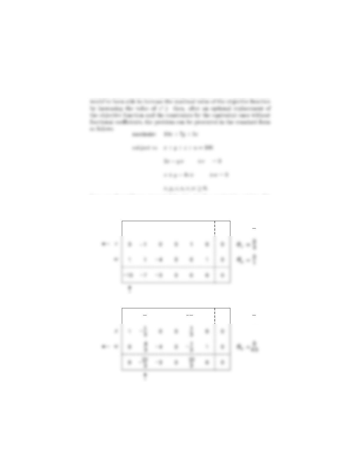
6. a. To simplify the task of getting an initial basic feasible solution here,
we can replace the equality constraint ++= 100 by the inequality
++≤100because an optimal solution (∗
∗
∗)to the problem
with the latter constraint must satisfy the former one.. (Otherwise, we
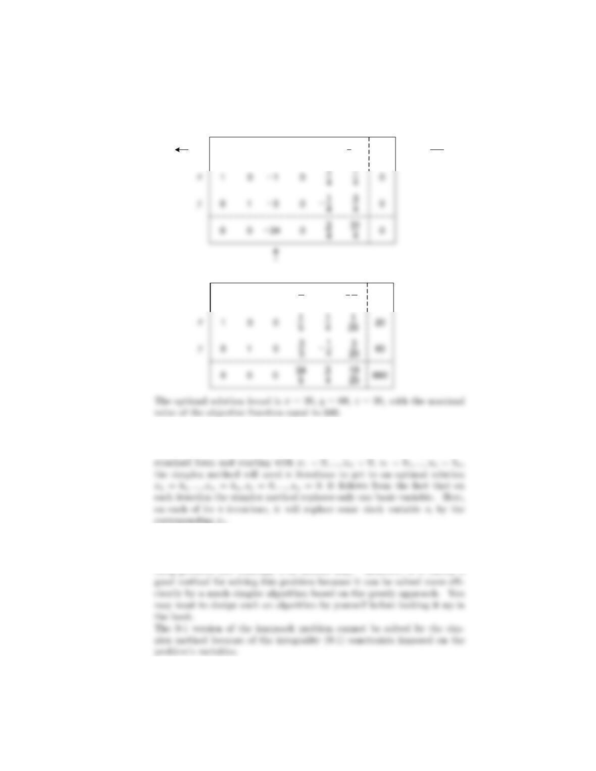
Here are the tableaux generated by the simplex method in solving this
problem:
zuvw
u
110010011
xy
~u=100
1
0
zuvw
u
11 01000
xy
~u=100
4/3
0
4
3
1
3
10
zuvw
u
51 0 1000
xy
~u=100
5
0
01
zuvw
z
10200
xy
~u=100
5
0
0
1
5
1
5
7. The optimal solution to the problem is 1=1 =After in-
troducing a slack variable in the th inequality =to get to the
8. The continuous version of the knapsack problem can be solved by the
simplex method, because it is a special case of the general linear program-
11
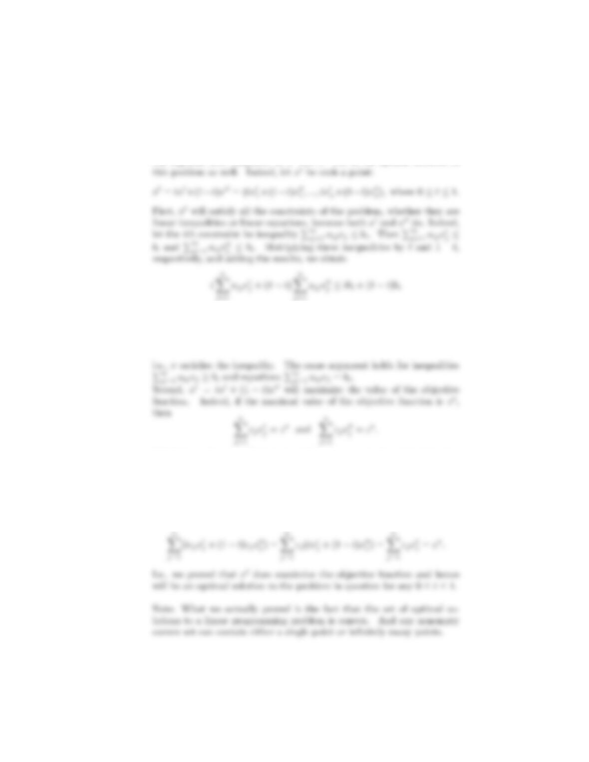
9. The assertion follows immediately from the fact that if 0=(0
1 0
)
and 00 =(00
1 00
)are two distinct optimal solutions to the same linear
programming problem, then any of the infinite number of points of the
line segment with endpoints at 0and 00 will be an optimal solution to
or
X
=1
( 0
+(1−) 00
)=
X
=1
(0
+(1−)00
)=
X
=1
≤
Multiplying these equalities by and 1−, respectively, and adding the
results, we will obtain
X
=1
0
+(1−)
X
=1
00
=∗+(1−)∗
or
12
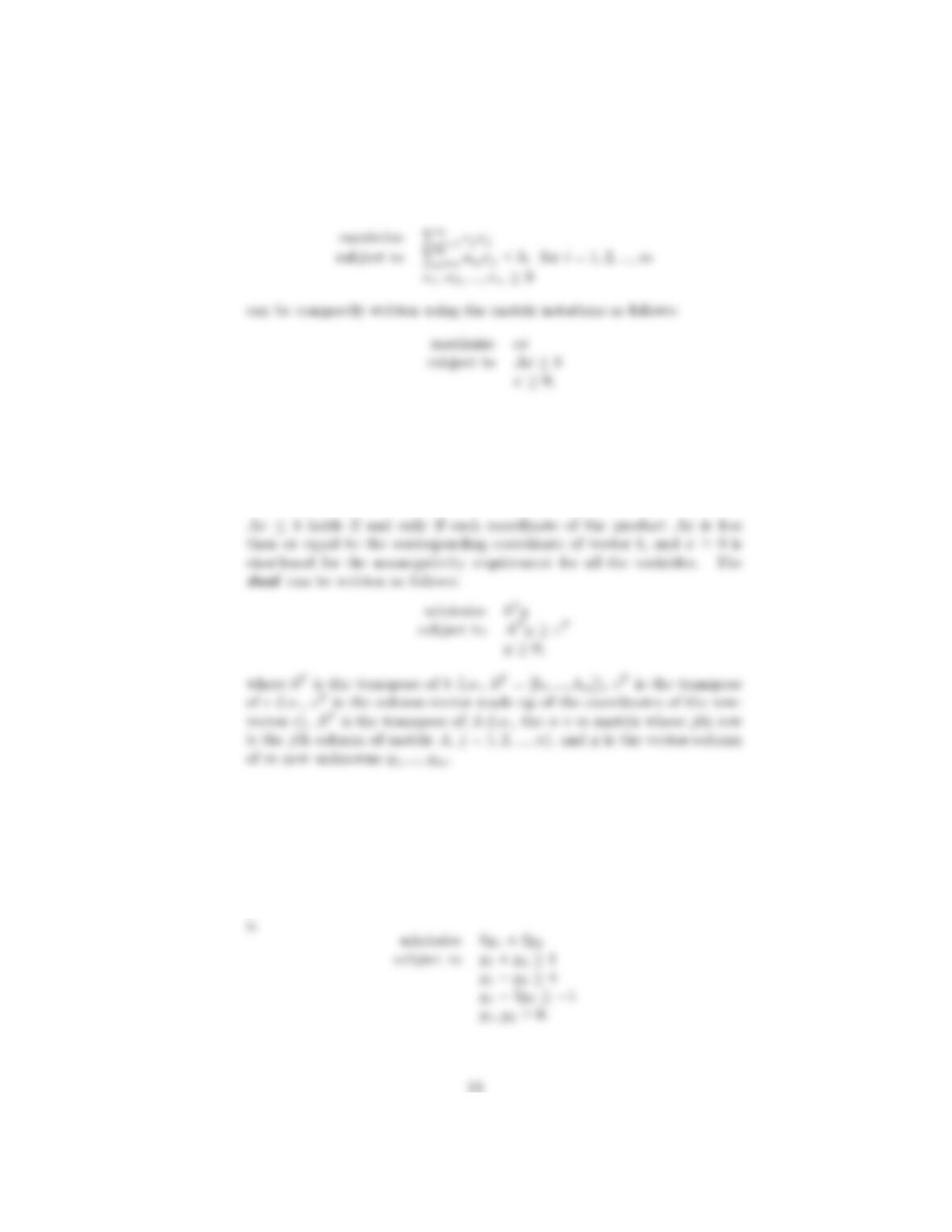
10. a. A linear programming problem
where
=£1 ¤=⎡
⎢
⎣
1
.
.
.
⎤
⎥
⎦=⎡
⎢
⎣
11 1
.
.
..
.
.
1
⎤
⎥
⎦=⎡
⎢
⎣
1
.
.
.
⎤
⎥
⎦
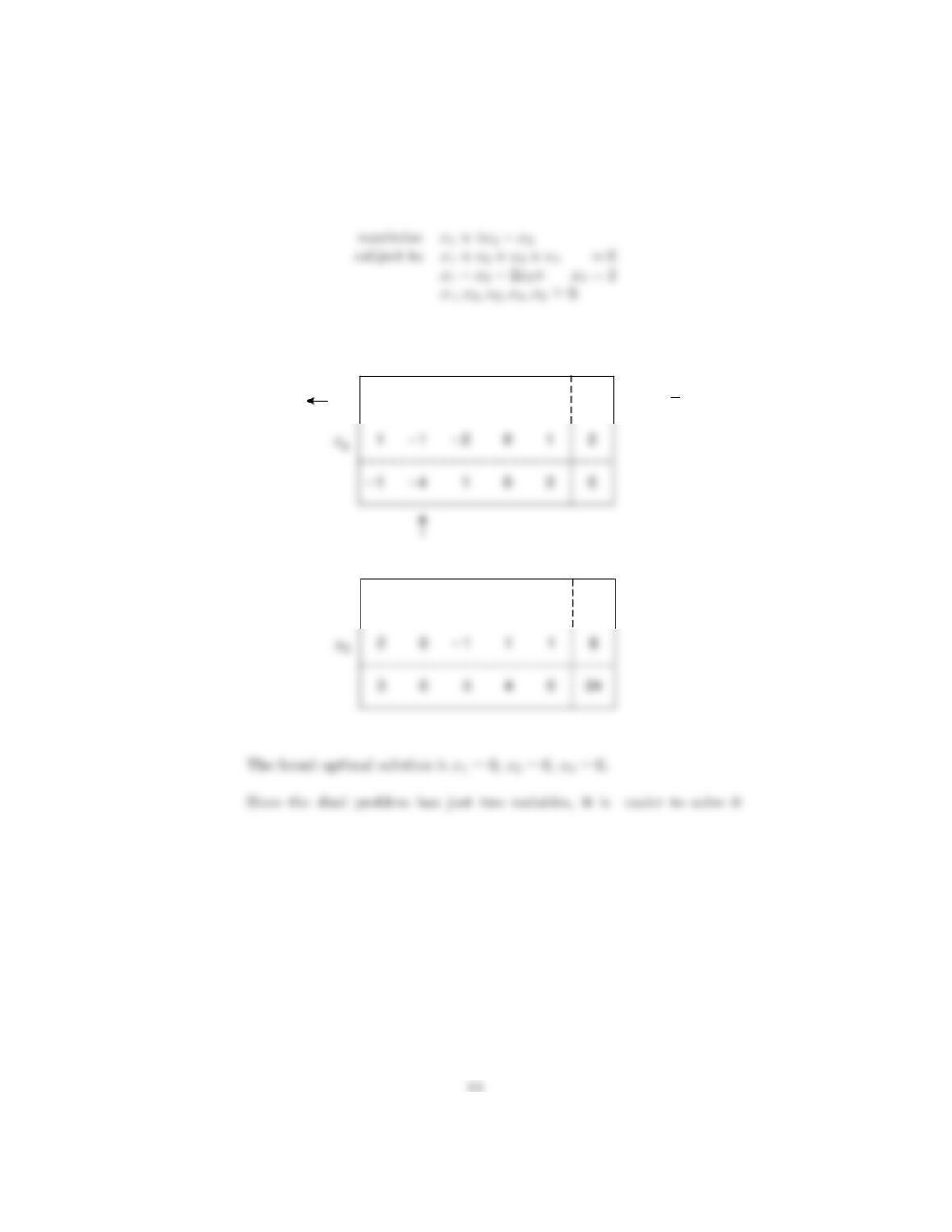
b. The dual of the linear programming problem
maximize 1+42−3
subject to 1+2+3≤6
1−2−23≤2
1
2
3≥0
c. The standard form of the primal problem is
The simplex method yields the following tableaux:
10
x
1
1234
xxx
116
x4
0~x=6
1
4
5
x
10
x
1
1234
xxx
116
x2
0~x=
6
2
4
5
x
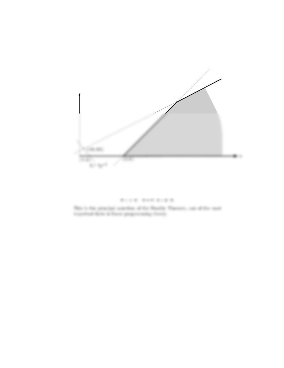
geometrically. Its feasible region is presented in the following figure:
y
( 9, 5 )
y – 2y = –1
2
12
y – y = 4
12
Although it is unbounded, the minimization problem in question does have
afinite optimal solution 1=4
2=0Note that the optimal values of
the objective functions in the primal and dual problems are equal to each
other:
15
Exercises 10.2
1. Since maximum-flow algorithms require processing edges in both direc-
tions, it is convenient to modify the adjacency matrix representation of a
2. Apply the shortest-augmenting path algorithm to find a maximum flow
and a minimum cut in the following networks:
a.
1 2 5
52
4
64
3. a. Does the maximum-flow problem always have a unique solution? Would
your answer be different for networks with different capacities on all their
edges?
4. a. Explain how the maximum-flow problem for a network with several
sources and sinks can be transformed to the same problem for a network
with a single source and a single sink.
16
root to the leaves. Design an efficient algorithm for finding a maximum
flow in such a network What is the time efficiency of your algorithm?
6. Ba. Prove equality (10.9).
7. a. Express the maximum-flow problem for the network of Figure 10.4 as
8. As an alternative to the shortest-augmenting-path algorithm, Edmonds
and Karp [Edm72] suggested the maximal-augmenting-path algorithm in
9. Write a report on a more advanced maximum-flow algorithm such as
(i) Dinitz’s algorithm, (ii) Karzanov’s algorithm, (iii) Malhotra-Kamar-
Maheshwari algorithm, or (iv) Goldberg-Tarjan algorithm.
10. Dining problem Several families go out to dinner together. To increase
their social interaction, they would like to sit at tables so that no two
members of the same family are at the same table. Show how to find
Hints to Exercises 10.2
1. What properties of the adjacency matrix elements stem from the source
and sink definitions, respectively?
4. a. Add extra vertices and edges to the network given.
b. If an intermediate vertex has a constraint on a flow amount that can
flow through it, split the vertex into two.
5. Take advantage of the recursive structure of a rooted tree.
8. n/a
9. n/a
18
Solutions to Exercises 10.2
1. The definition of a source implies that a vertex is a source if and only if
there are no negative elements in its row in the modified adjacency matrix.
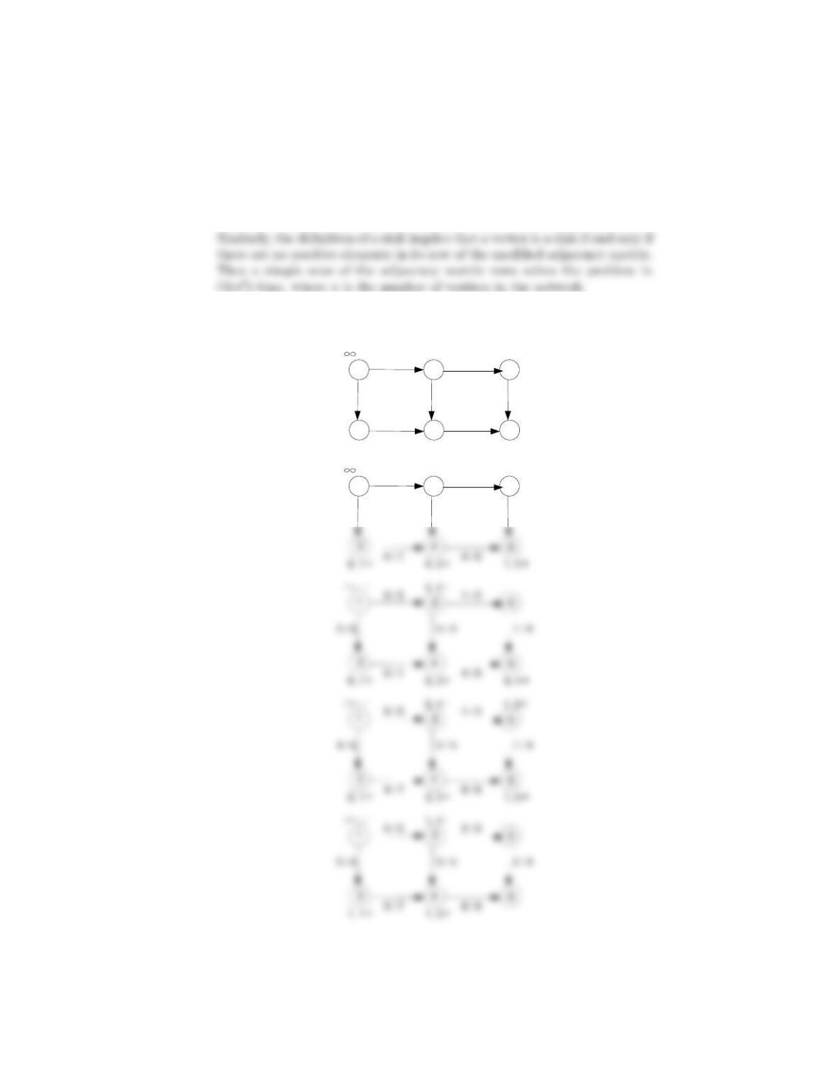
2. a. Here is an application of the shortest-augmenting path algorithm to
the network of Problem 2a:
1 2 5
36
4
0 / 5 0 / 2
0 / 4
0 / 8
0 / 7
0 / 6 0 / 4
, – 2, 2+
4, 4 +
4, 2+
5, 1 +
6, 1+
1 2 5
4 / 5 0 / 2
0 / 4
0 / 6 4 / 4
, – 1, 2+
1, 1 +
19
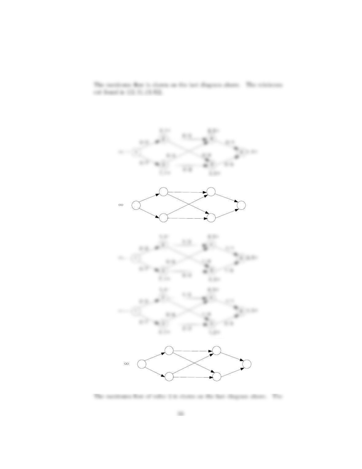
b. Here is an application of the shortest-augmenting path algorithm to
the network of Problem 10.2b:
2 4
3 5
1 / 3
0 / 2
1 6
1 / 1
1 / 2
0 / 7 0 / 5
1, 1+1, 2 +
0 / 4 0 / 4 1, 5 +
1, 2 +
7, 1 +
_
,
2 4
3 5
0 / 3
2 / 2
1 6
1 / 1
2 / 2
3 / 7 4 / 5
3, 3 +
1 / 4 2 / 4
4 ,1 +
_
,