CHAPTER 10
Compressibility and Settlement
QUESTIONS AND PRACTICE PROBLEMS
Section 10.2 Changes in Vertical Effective Stress
10.1 The current σz′ at a certain point in a saturated clay is 181 kPa. This soil is to be covered
with a 2.5 m thick fill that will have a unit weight of 19.3 kN/m3. What will be the value
of σz′ at this point immediately after the fill is placed, before any consolidation has
occurred? What will it be after the consolidation settlement is completed?
Solution
Immediately after the fill is placed, its weight will be carried entirely by the pore water
10.2 A circular tank 50 feet in diameter is constructed on top of a saturated soil with a
saturated unit weight of 112 lb/ft3. The total weight of the tank when filled is 6,125 k.
The groundwater table is at the ground surface. Compute σ‘z a point 25 feet below the
center of the tank immediately after the tank is placed and filled, before any consolidation
has occurred. What will σ‘z be at the same point after consolidation settlement is
completed?
Solution
Before placement of the tank the effective vertical stress is
10-2 Compressibility and Settlement Chap. 10
Using Figure 9.13
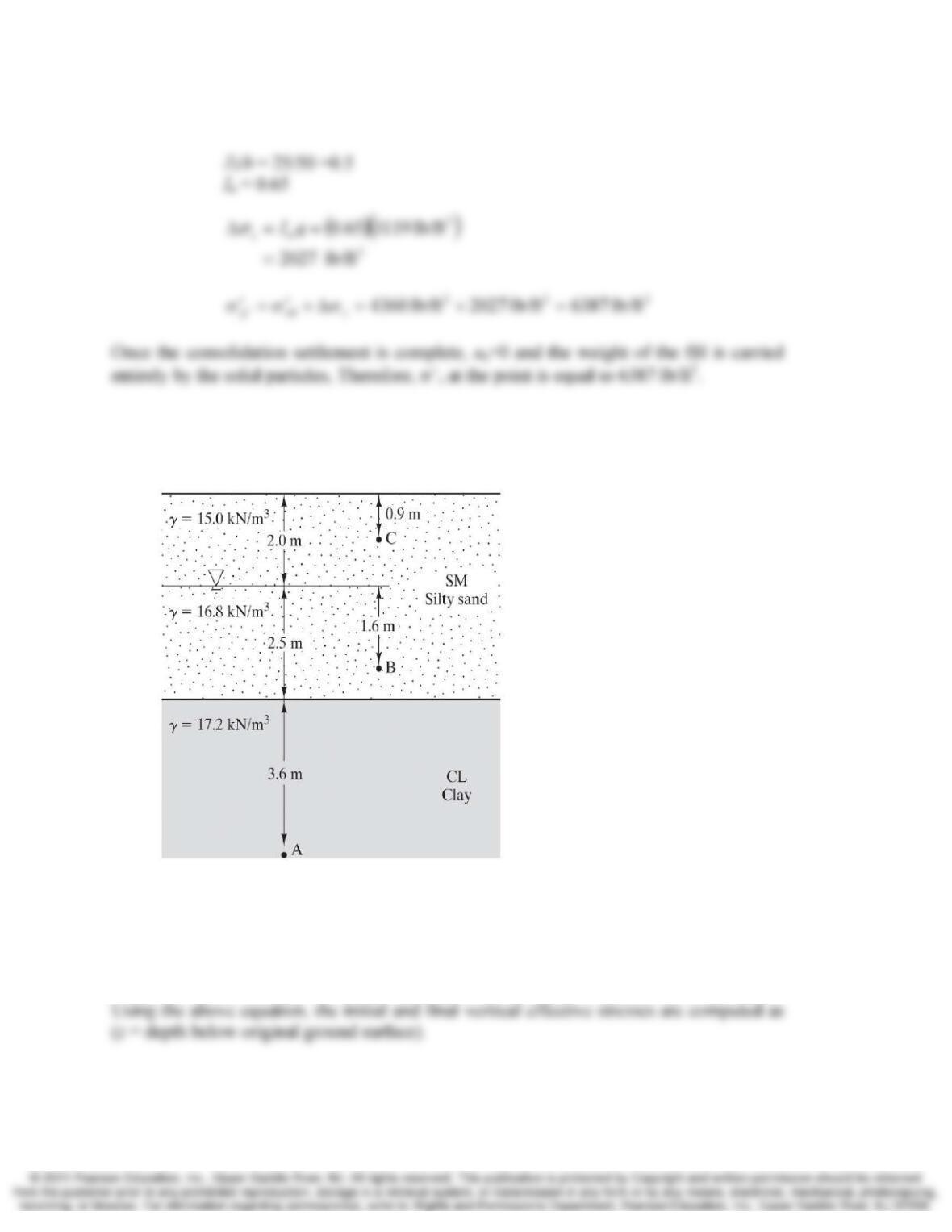
10.3 A 4.0 m thick fill with a unit weight of 20.1 kN/m3 is to be placed on the soil profile
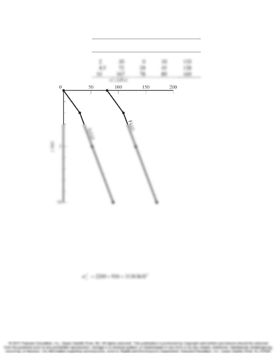
shown in Figure 9.11. Develop plots of σ′z0 and σ′zf vs. depth. The plot should extend
from the original ground surface to a depth of 10.0 m.
Figure 9.11 Soil profile for Example 9.2.
Solution
(
)
(
)
kPa 80m 4.0kN/m 20.1 0
3
00 +
′
=+
′
=+
′
=
′zzfillfillzzf H
σσγσσ
Chap. 10 Compressibility and Settlement 10-3
z
(m)
σ
z
(kPa) u
(kPa)
σ
‘z0
(kPa)
σ
‘zf
(kPa)
0 0 0 0 80
10.4 The groundwater table at a certain site was at a depth of 10 ft below the ground surface,
and the vertical effective stress at a point 30 ft below the ground surface was 2200 lb/ft2.
Then a series of wells were installed, which caused the groundwater table to drop to a
depth of 25 ft below the ground surface. Assuming the unit weight of the soil above and
below the groundwater table are equal, compute the new σz′ at this point.
Solution
(
)
(
)
2
lb/ft 9364.621025 =−=Δ=
′
Δu
z
σ
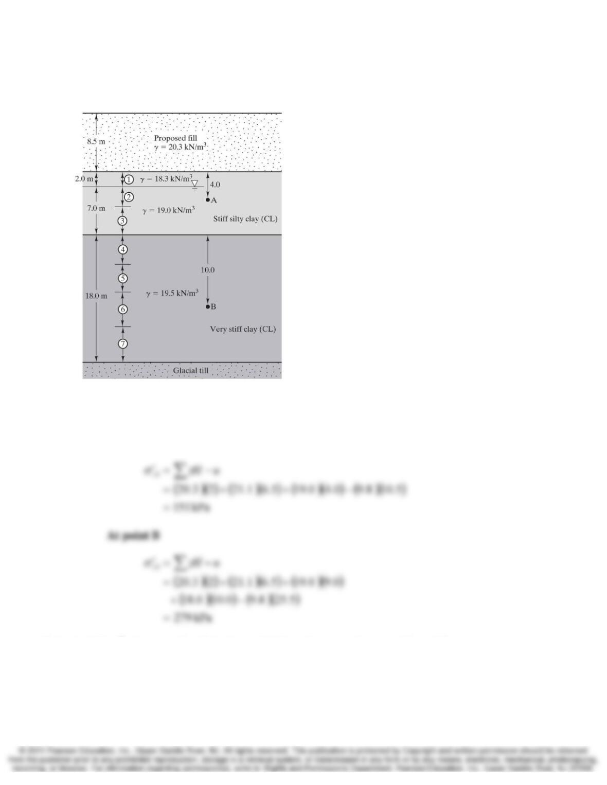
10.5 The fill shown in Figure 10.21 was placed many years ago and consolidation in both clay
layers due to the fill placement has is complete. The fill was placed near a river that has
since been dammed. Filling of the reservoir behind the dam has raised the local
groundwater table to a point 2 m below the ground surface. The raising of the water table
has been slow and has not induced any excess pore pressures in the clay soils. Compute
10-4 Compressibility and Settlement Chap. 10
σz′ at points A and B due to the rise of the groundwater table. Assume the saturated unit
weight of the fill material is 21.1 kN/m3
Figure 10.21 Soil profile for Example 10.6.
Solution
At point A
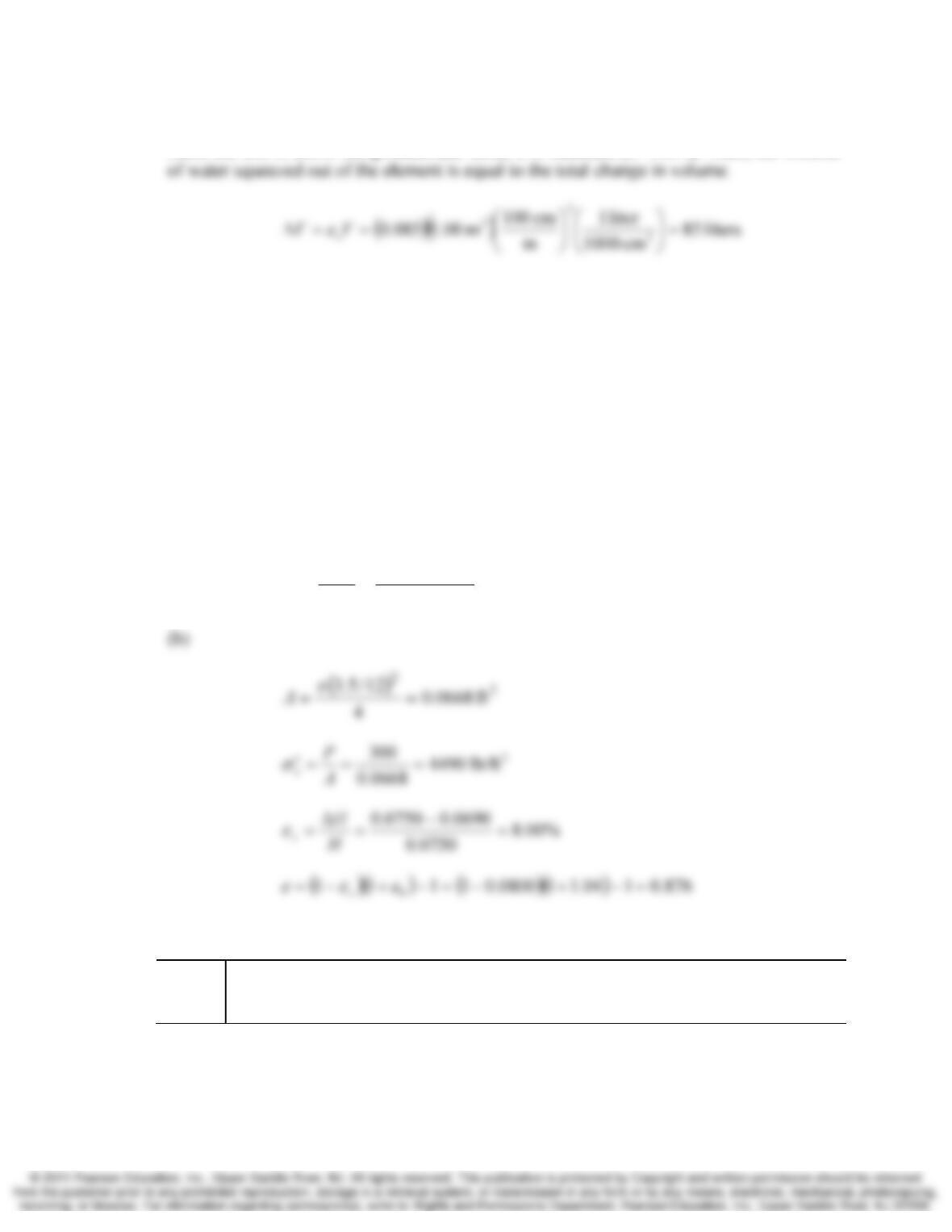
10.6 A 1.00 m3 element of soil is located below the groundwater table. When a new
compressive load was applied, this element consolidated, producing a vertical strain, εz,
of 8.5%. The horizontal strain was zero. Compute the volume of water squeezed out of
this soil during consolidation and express your answer in liters.
Chap. 10 Compressibility and Settlement 10-5
Solution
Since the soil is below the groundwater table, it is saturated (S=100%). Thus, the volume
Section 10.5 Consolidation Test
10.7 A consolidation test is being performed on a 3.50 in diameter saturated soil sample that
had an initial height of 0.750 in and an initial moisture content of 38.8%.
(a) Using Gs = 2.69, compute the initial void ratio, e0.
(b) At a certain stage of the test, the normal load P was 300 lb. After the consolidation at
this load was completed, the sample height was 0.690 in. Compute σz′ (expressed in
lb/ft2), εz, and e.
Solution
(a)
()
(
)
1.04
1
69.2388.0
0=== S
wG
es
10.8 A consolidation test of a soft marine silty clay produced the following data
σz′
(lb/ft2) 50 250 500 1000 2000 4000 8000 16,000 4000 500
εz 0.007 0.028 0.059 0.097 0.145 0.189 0.235 0.278 0.271 0.253
The initial void ratio of the sample was 1.24 and σz0′ at the sample depth was 270 lb/ft2
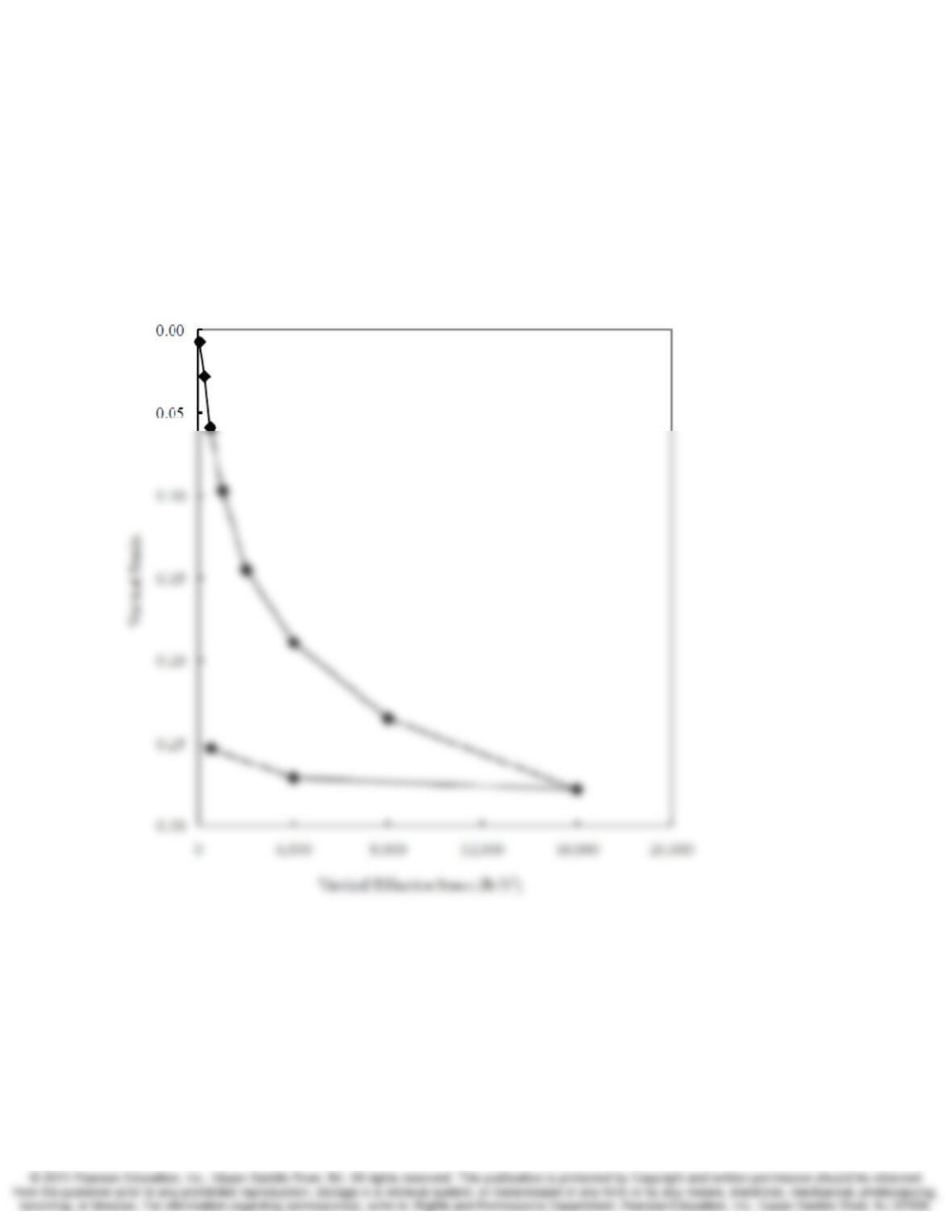
(a) Plot these data on an arithmetic diagram similar to that in Figure 10.10(a)
10-6 Compressibility and Settlement Chap. 10
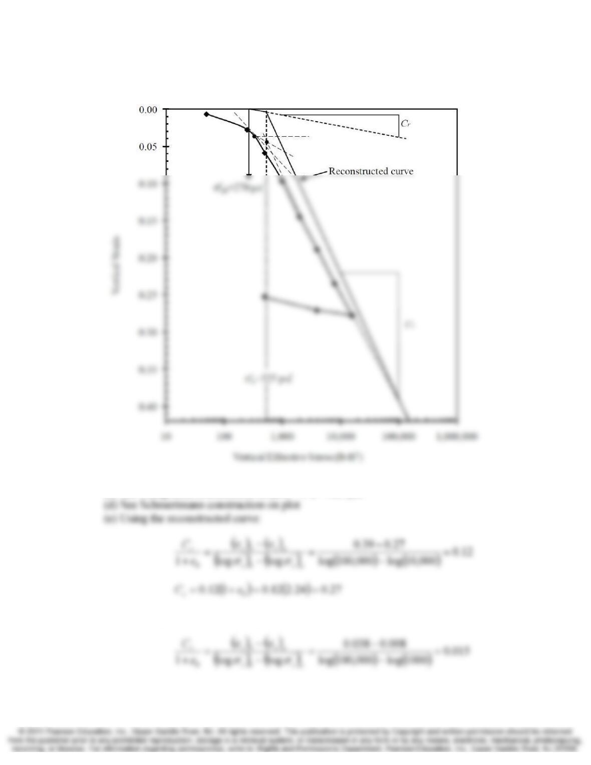
(b) Plot these data on a semilogarithmic diagram similar to that in Figure 10.10(b)
(c) Using Casagrande’s method, find σ‘c
(d) Using Schmertmann’s method adjust the test results
(e) Determine Cc and Cr
(f) The soil has a plasticity index of 17. Based on Kulhawy and Mayne’s correlations, do
the consolidation test results seem reasonable?
Solution
(a)
Chap. 10 Compressibility and Settlement 10-7
(b)
(c) See Casagrande construction on plot – σ’c = 525 psf
Using the original decompression curve:
10-8 Compressibility and Settlement Chap. 10
(f) Per Kulhawy and Mayne’s correlation:
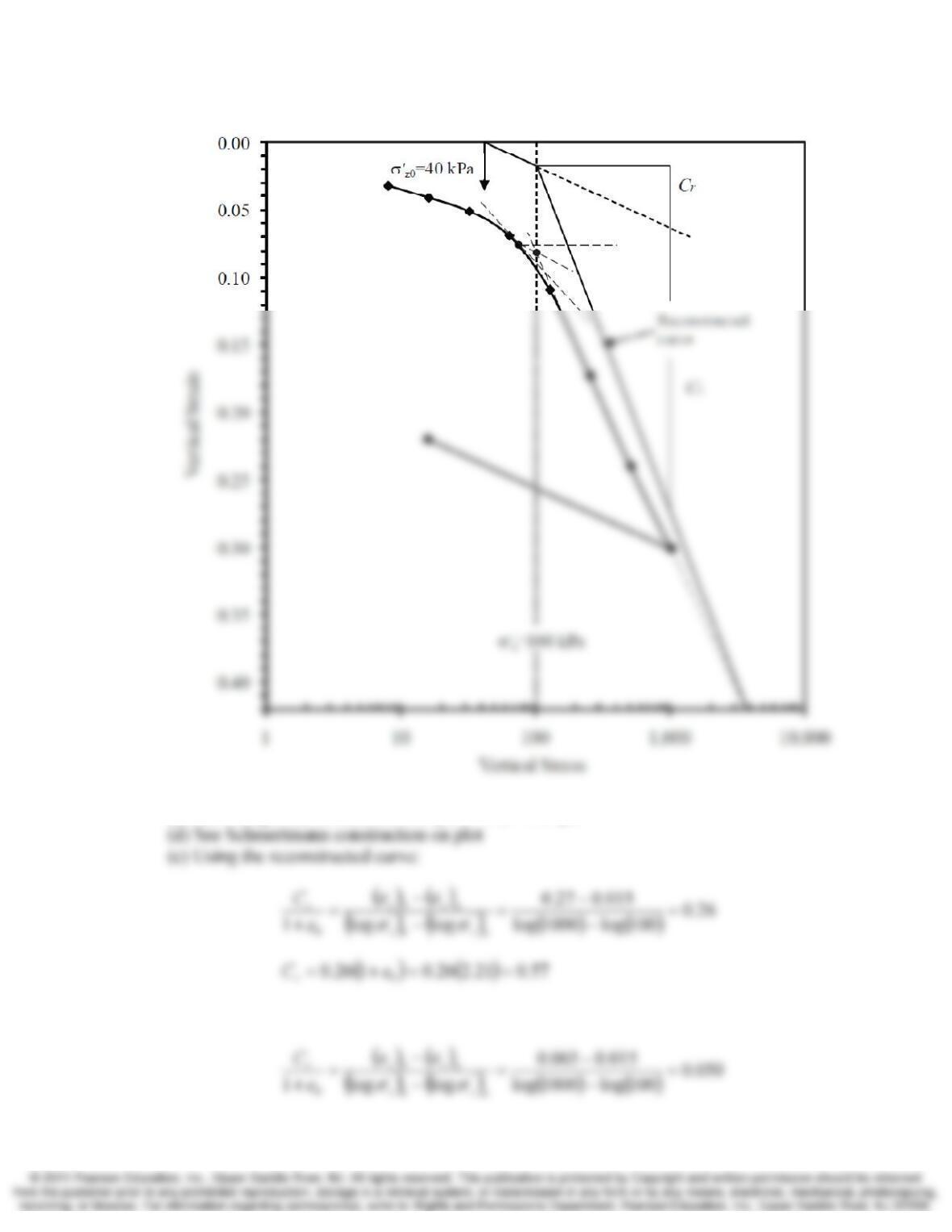
10.9 A consolidation test on a sample of clay produced the following data:
σ
z
′ (kPa) 8 16 32 64 128 256 512 1024 16
ε
z
0.032 0.041 0.051 0.069 0.109 0.173 0.240 0.301 0.220
The initial void ratio of the sample was 1.21, and σz0′ at the sample depth was 40 kPa.
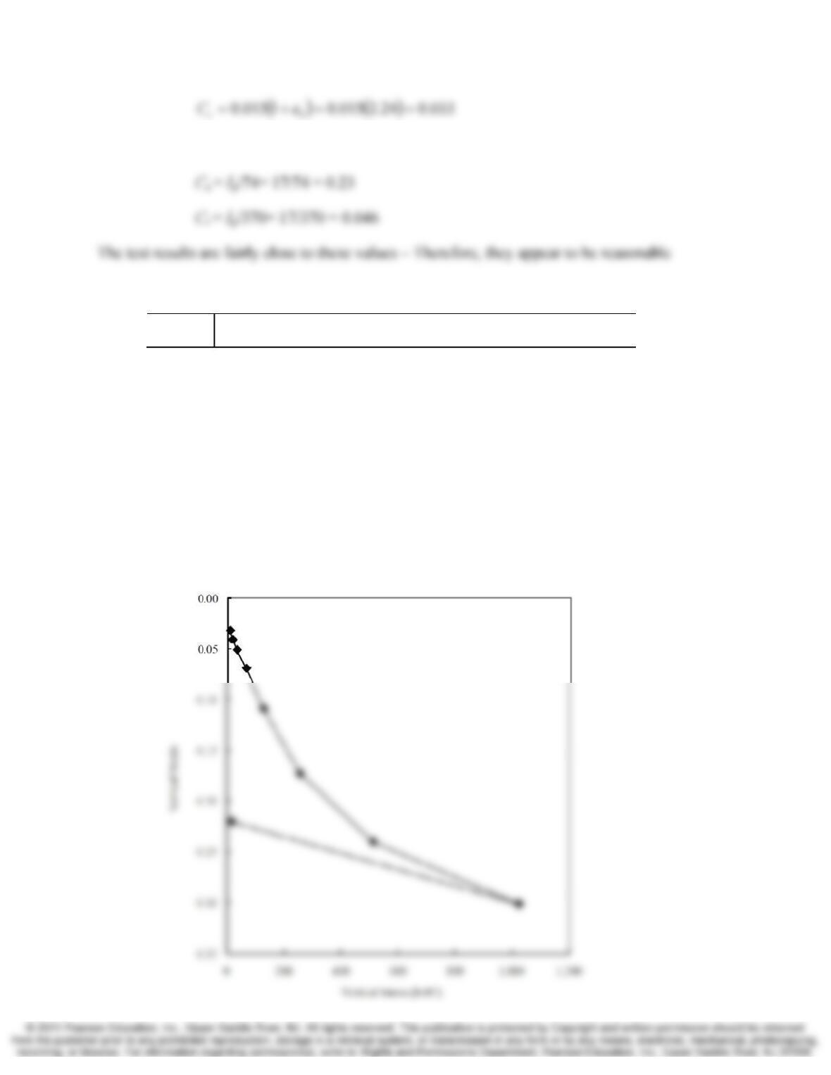
(a) Plot these data on an arithmetic diagram similar to that in Figure 10.10(a)
(b) Plot these data on a semilogarithmic diagram similar to that in Figure 10.10(b).
(c) Using Casagrande’s method, find σc′.
(d) Using Schmertmann’s method, adjust the test results.
(e) Determine Cc and Cr.
(f) The soil has a plasticity index of 23. Based on Kulhawy and Mayne’s correlations,
do the consolidation test results seem reasonable?
Solution
(a)
Chap. 10 Compressibility and Settlement 10-9
(b)
(c) See Casagrande construction on plot – σ’c = 525 psf
Using the original decompression curve:
10-10 Compressibility and Settlement Chap. 10
()
(
)
0.1121.2050.01050.0 0
=
=+= eCr
(f) Per Kulhawy and Mayne’s correlation:
Section 10.6 Consolidation Status in the Field
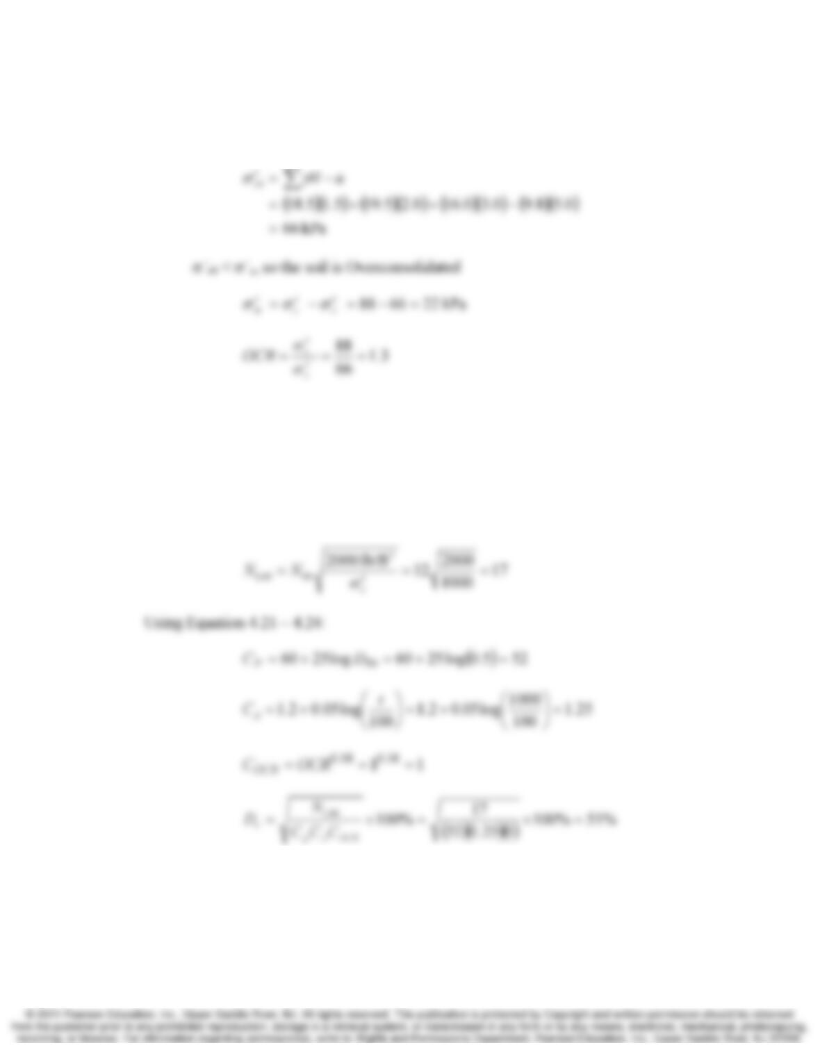
10.10 Before the placement of any fill, a consolidation test was performed on a soil sample
obtained from Point B in Figure 10.20. The measured preconsolidation stress was 88 kPa.
Determine whether the soil is normally consolidated or overconsolidated, then compute
the overconsolidation margin and overconsolidation ratio at Point B.
Note: These computations are based on the initial conditions, and thus should not
include the weight of the proposed fill.
Figure 10.20 Soil profile for Example 10.5
Chap. 10 Compressibility and Settlement 10-11
Solution
At point B:
10.11 A saturated, normally consolidated, 1000-year-old fine-to-medium sand has an SPT
N60 = 12 at a depth where the vertical effective stress is about 1000 lb/ft2 and D50 =
0.5 mm. Using the techniques described in Chapters 3 and 4, determine the relative
density of this soil, then estimate Cc/(1+e0) based on Table 10.4.
Solution
Using Equation 3.2:
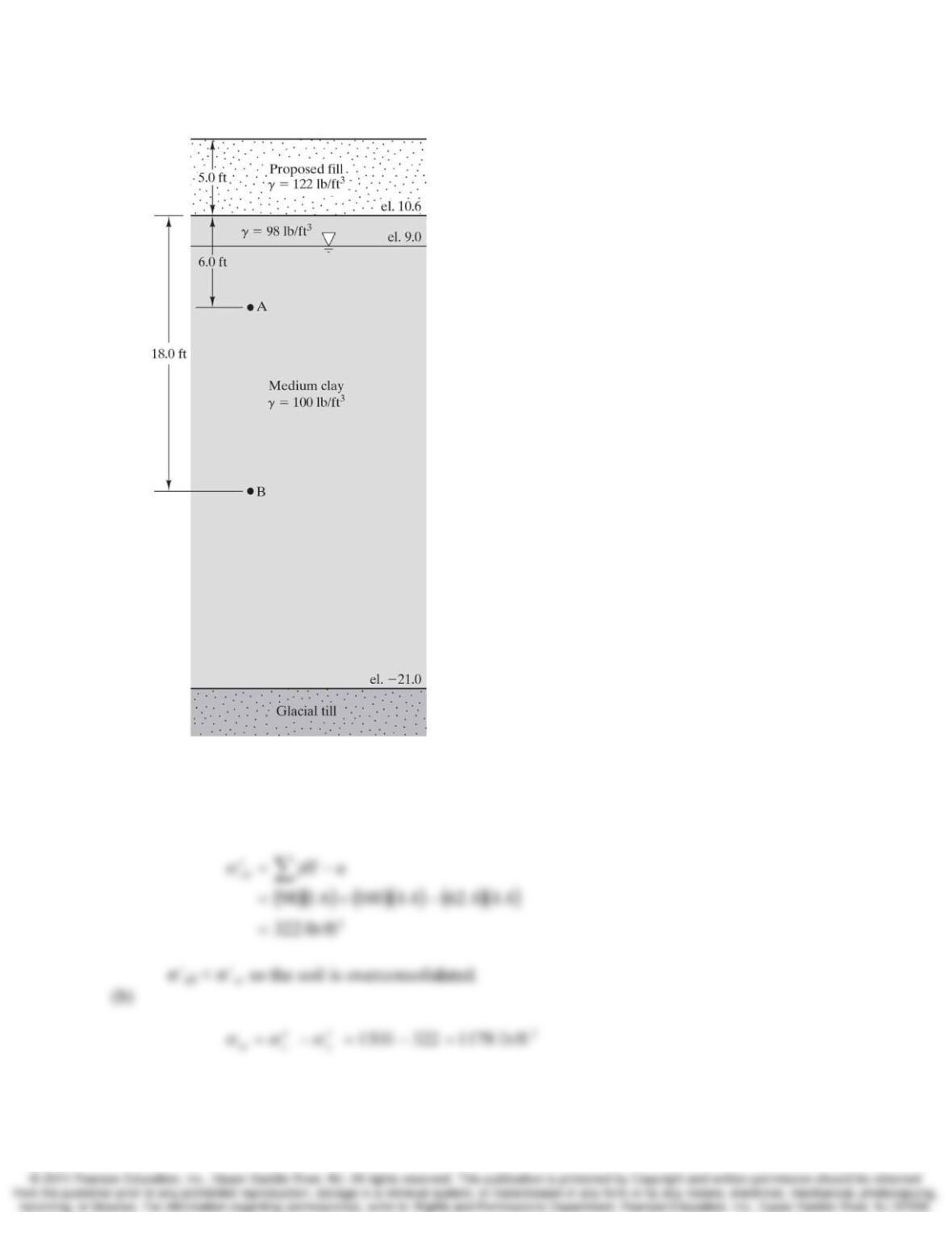
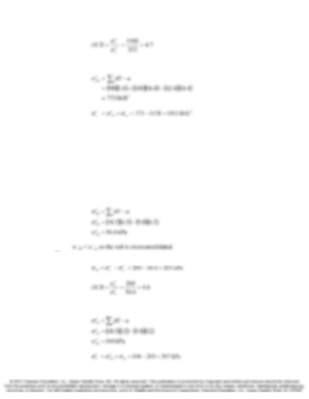
10.12 A consolidation test has been performed on a sample obtained from Point A in
Figure 10.3. The measured preconsolidation stress was 1500 lb/ft2.
(a) Determine if the soil is normally consolidated or overconsolidated
(b) Compute the overconsolidation margin and the overconsolidation ratio
10-12 Compressibility and Settlement Chap. 10
(c) Compute σc′ at Point B
Figure 10.3 Soil profile for Example 10.1. el. = elevation.
Solution
(a) At Point A:
Chap. 10 Compressibility and Settlement 10-13
(c) At Point B:
10.13 A consolidation test has been performed on a sample obtained from a saturated clay at a
point 6.5 m below the ground surface. The groundwater table is at the ground surface and
the unit weight of the clay is 18.5 kN/m3. The measured preconsolidation stress was
260 kPa.
(a) Determine if the soil is normally consolidated or overconsolidated
(b) Compute the overconsolidation margin and the overconsolidation ratio
(c) Compute σc′ at depth of 12 m in the same soil.
Solution
(a) At a point 6.5m below ground surface:
(b)
(c) At a point 12 m below the ground surface:
10-14 Compressibility and Settlement Chap. 10
10.14 Laboratory consolidation test for all soils have both a recompression curve and a virgin
curve. This is true even for normally consolidated soils. Explain how the lab test for a
normally consolidated soil can have a recompression curve even though the soil in the
field has never been preloaded.
Solution
During the process of sampling the soil removed from the field is unloaded from its in
Section 10.8 Consolidation Settlement Predictions
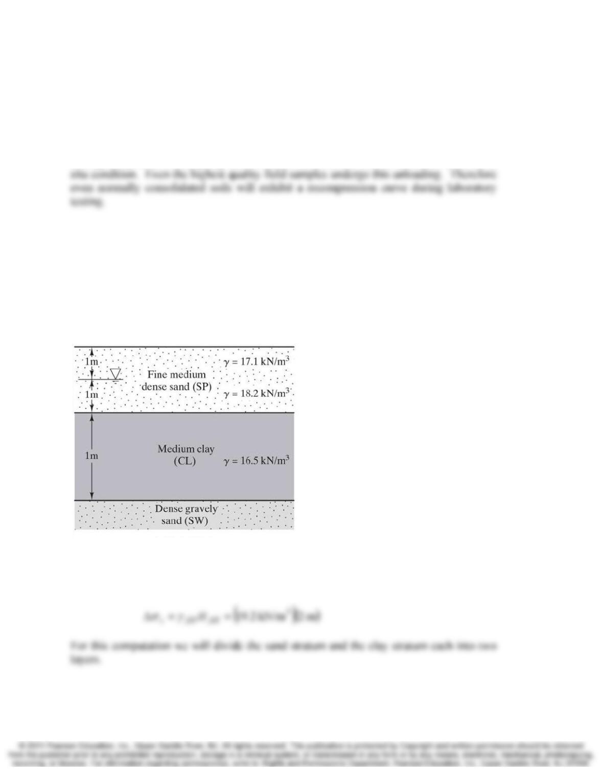
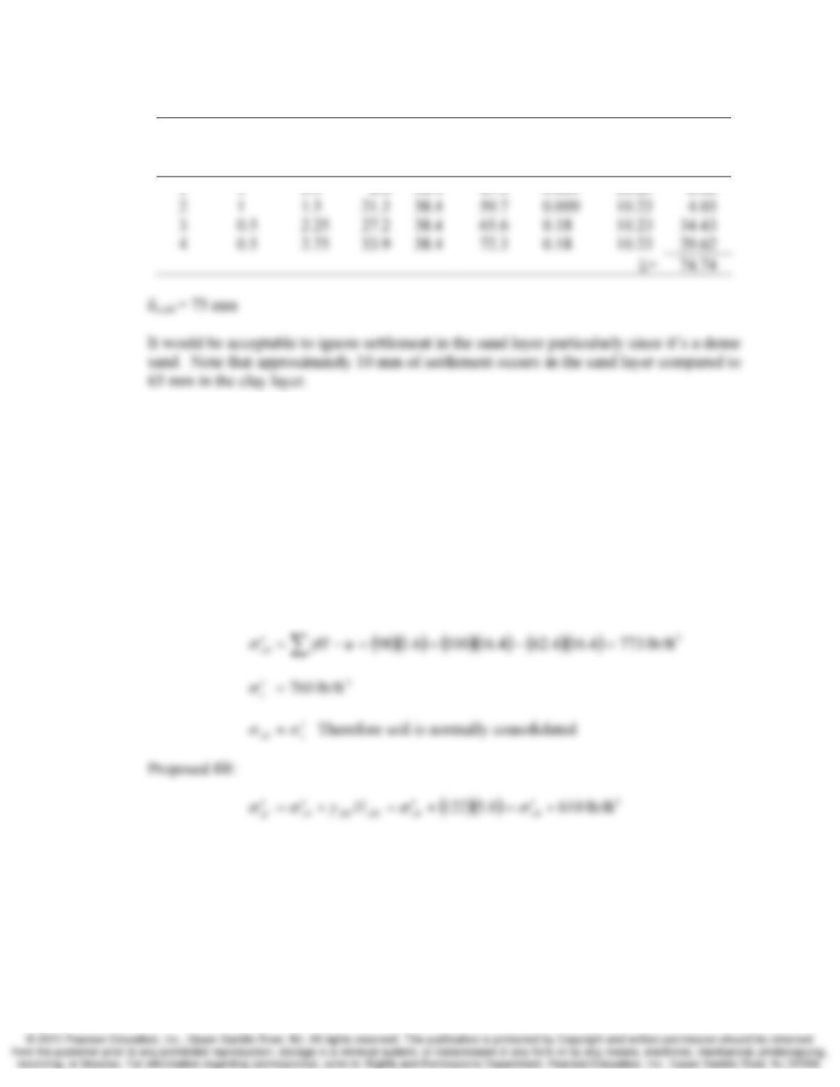
10.15 A 2 m thick fill with an in place unit weight of 19.2 kN/m3 is to be placed on top of the
soil profile shown in Figure 10.25. Both the sand and the clay are normally consolidated.
The sand is fine, poorly graded and medium dense with Cc/(1+e0) estimated to be 0.009.
Lab consolidation tests on the clay produced Cc/(1+e0) = 0.18. Compute the total
consolidation settlement due to the placement of the fill. Would it be acceptable to ignore
the settlement generated by consolidation of the sand layer?
Figure 10.25 Soil Profile for Problem 10.15.
Solution
Applied stress from the proposed fill
Chap. 10 Compressibility and Settlement 10-15
Layer H (m) zf
At midpoint of layer
Cc/(1+e0) Eqn.
δc,ult
(mm)
σ
‘z0
(kPa)
Δ
σz
(kPa)
σ
‘zf
(kPa)
10.16 A 5.0 ft thick fill is to be placed on the soil profile as shown in Figure 10.3. A
consolidation test performed on a sample obtained from Point B produced the following
results: Cc = 0.27, Cr = 0.10, e0 = 1.09, σc′ = 760 lb/ft2. Compute the ultimate
consolidation settlement due to the weight of this fill and determine the ground surface
elevation after the consolidation is complete.
Note: The first layer in your analysis should extend from the original ground
surface to the groundwater table.
Solution
At sample B:
10-16 Compressibility and Settlement Chap. 10
Layer
H
(ft) zf
At midpoint of layer
Cc/(1+e0)Eqn.
δc,ult
(ft)
σ‘z0
(psf)
Δ
σz
(psf)
σ
‘zf
(psf)
1 1.6 0.8 78.0 610 688.0 0.129 10.23 0.20
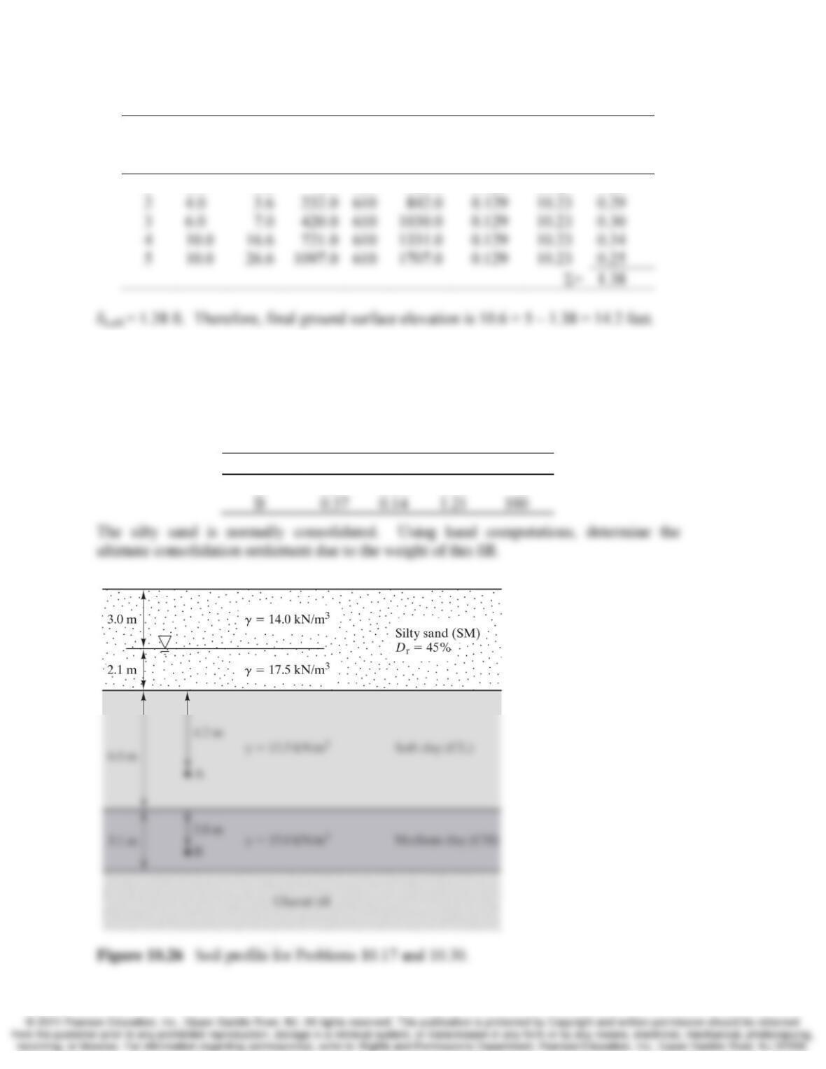
10.17 A 4.0 m thick fill is to be made of a soil with a Proctor maximum dry unit weight of
19.4 kN/m3 and an optimum moisture content of 13.0%. This fill will be compacted at
optimum moisture content to an average relative compaction of 92%. The underlying
soils are as shown in Figure 10.26. Consolidation tests were performed at Points A and B,
with the following results:
Sample Cc C
r
e0 σc
′
(kPa)
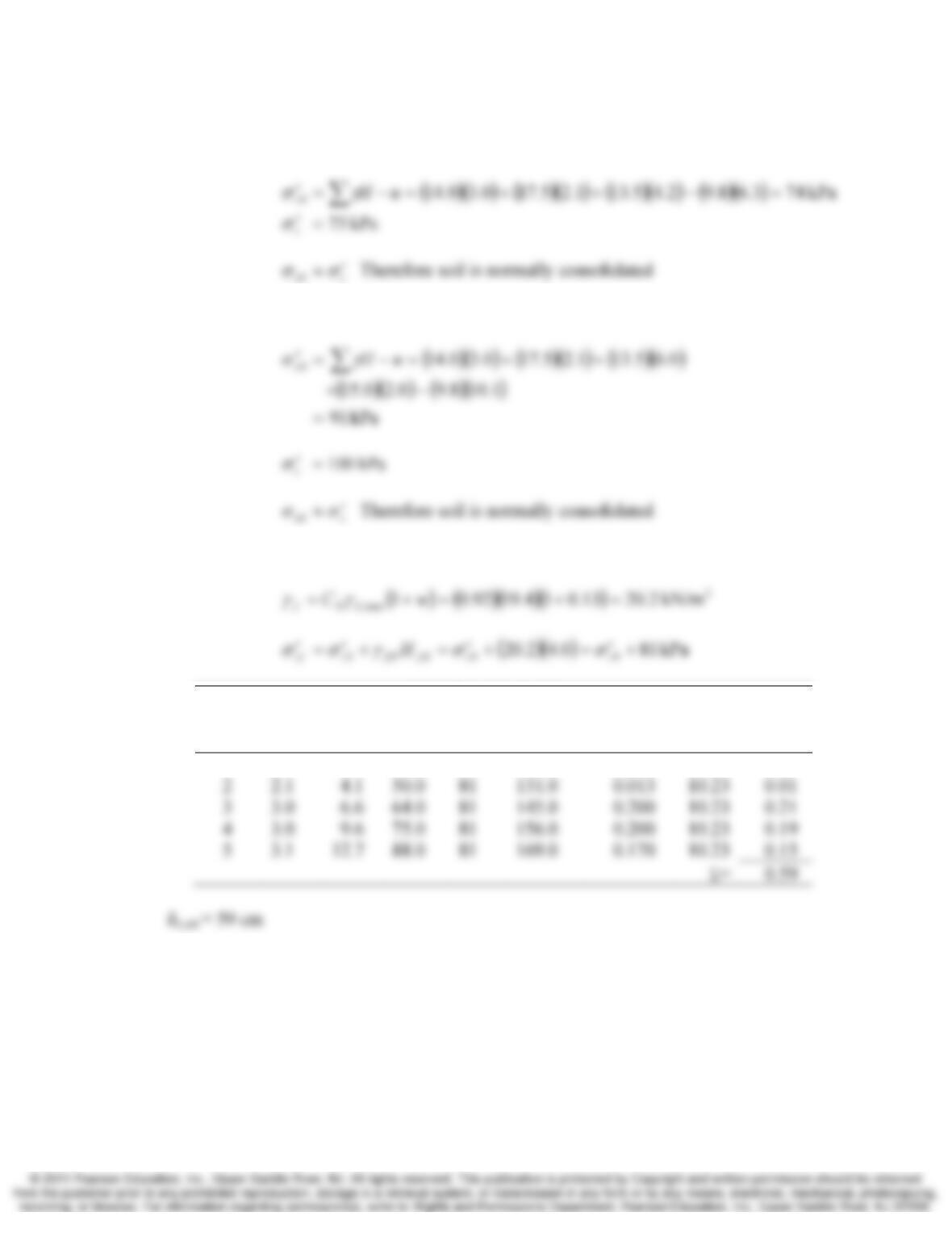
A 0.59 0.19 1.90 75
Σ
Chap. 10 Compressibility and Settlement 10-17
Solution
At sample A:
At sample B:
Proposed fill:
Layer
H
(m) zf
At midpoint of layer
Cc/(1+e0) Eqn.
δc,ult
(m)
σ
‘z0
(kPa)
Δ
σ
z
(kPa)
σ
‘zf
(kPa)
1 3.0 1.5 21.0 81 102.0 0.013 10.23 0.03
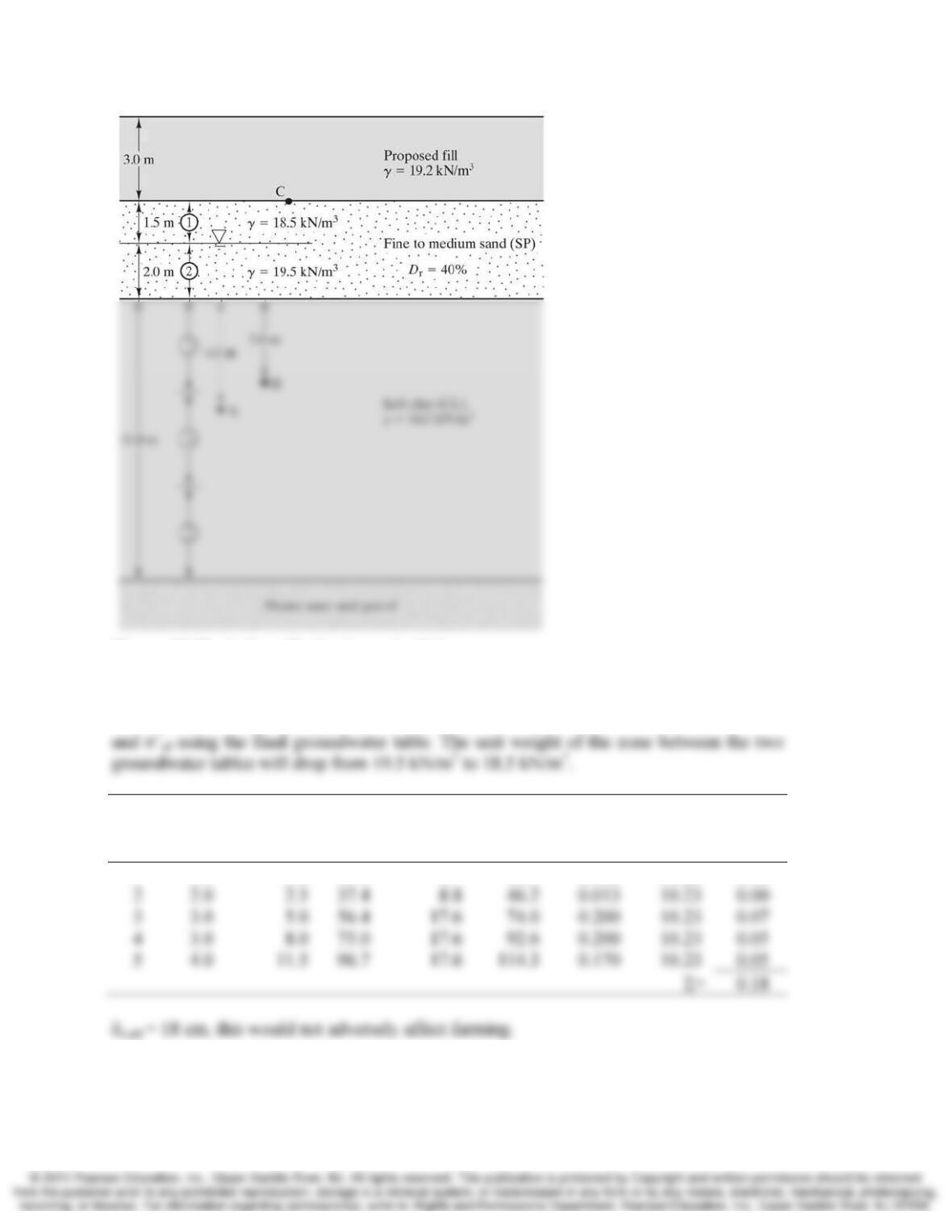
10.18 The owner of the land shown in the profile in Example 10.5 has decided not to build the
proposed fill. Instead, the land will be used for farming. To provide irrigation water, a
series of shallow wells will be drilled into the sand, and these wells will cause the
groundwater table to drop to the bottom of the sand layer (i.e., 2.0 m below its current
position). Compute the ultimate consolidation settlement due to this drop in groundwater.
Do you think such a settlement will adversely affect the farming?
10-18 Compressibility and Settlement Chap. 10
Figure 10.20 Soil profile for Example 10.5
Solution
Compute σ’z0 using the original groundwater table (same value as used in Example 10.5)
Layer H (m) zf
At midpoint of layer
Cc/(1+e0)Eqn.
δc,ult
(m)
σ‘z0
(kPa)
Δ
σ
z
(kPa)
σ
‘zf
(kPa)
1 1.5 0.8 13.9 0 13.9 0.013 10.23 0.00
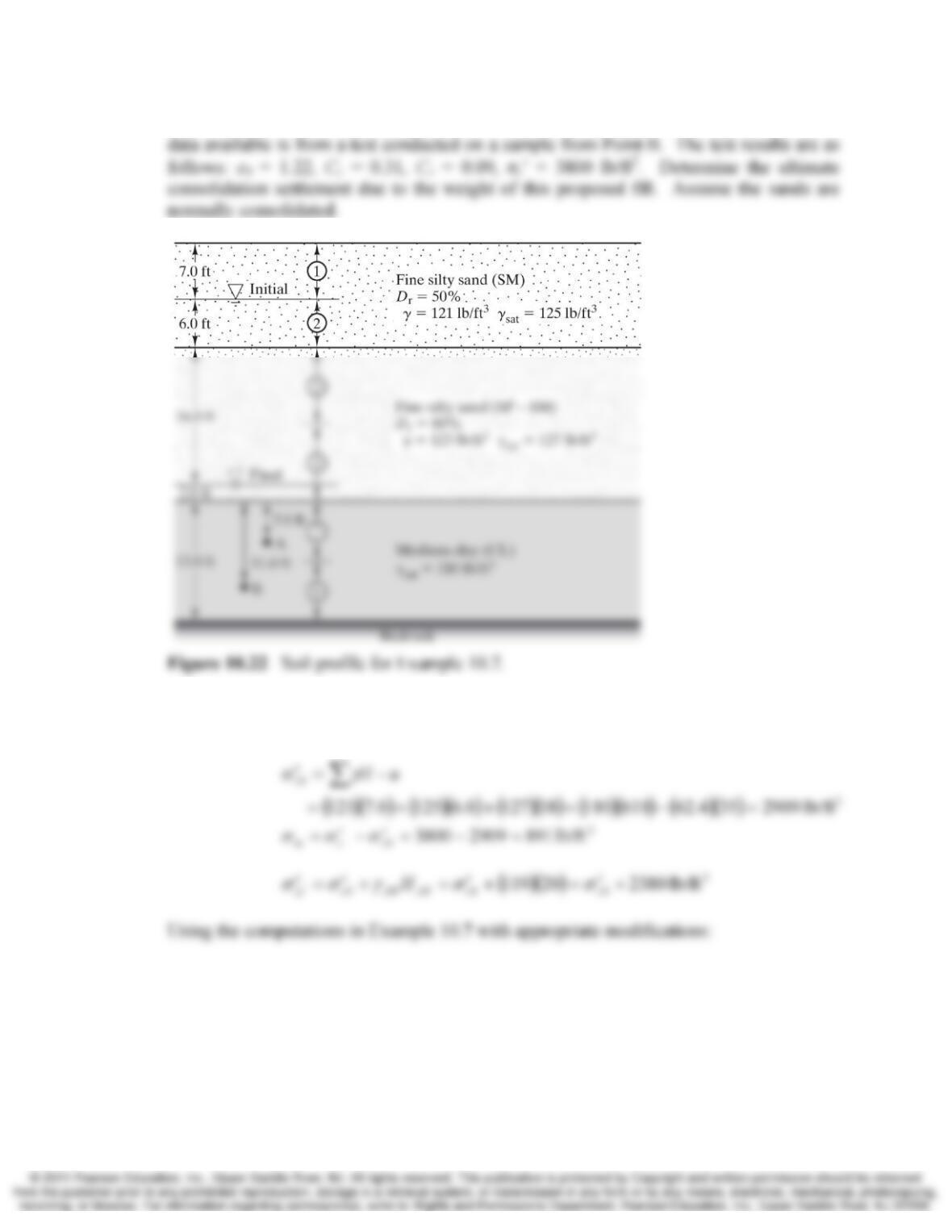
10.19 A certain site is underlain by the soil profile shown in Figure 10.22 with the groundwater
table at the initial location. The groundwater table will remain at this location, but a
Chap. 10 Compressibility and Settlement 10-19
20.0-ft deep fill with a unit weight of 119 lb/ft3 is to be placed. The only consolidation
Solution
At sample B: