Chapter 10: Production and Cost Estimation
Chapter 10:
PRODUCTION AND COST ESTIMATION
Essential Concepts
1. The cubic empirical specification for a short-run production function is derived from a long-run cubic
Q aK L bK L= +
2. The properties of a short-run cubic production function
( )Q AL BL= +
3 2
are:
a. Holding capital constant at
K
units, the short-run cubic production function is derived as follows:
b. The average and marginal products of labor are respectively
c. Marginal product of labor begins to diminish beyond Lm units of labor and average product of
labor begins to diminish beyond La units of labor, where
d. In order to have the necessary properties of a production function, the parameters must satisfy the
following restrictions:
3. To estimate a cubic short-run production function using linear regression analysis, you must first
transform the cubic equation into linear form:
4. Short-run cost functions should be estimated using data for which the level of usage of one or more of
5. Collecting data may be complicated by the fact that accounting data are based on expenditures and
6. The effects of inflation on cost data must be eliminated. To adjust nominal cost figures for inflation,
divide each observation by the appropriate price index for that time period.
Chapter 10: Production and Cost Estimation
7. The properties of a short-run cubic cost function
2 3
( )TVC aQ bQ cQ= + +
are:
f. In the short-run cubic specification, input prices are assumed to be constant and are not explicitly
included in the cost equation.
Summary of Short-Run Empirical Production and Cost Functions
Short-run cubic production
equations
Total product
Q = AL3 + BL2
Average product of labor
AP = AL2 + BL
Marginal product of labor
Restrictions on parameters
Total variable cost
TVC = aQ + bQ2 + cQ3
Average variable cost
AVC = a + bQ + cQ2
Restrictions on parameters
Chapter 10: Production and Cost Estimation
Answers to Applied Problems
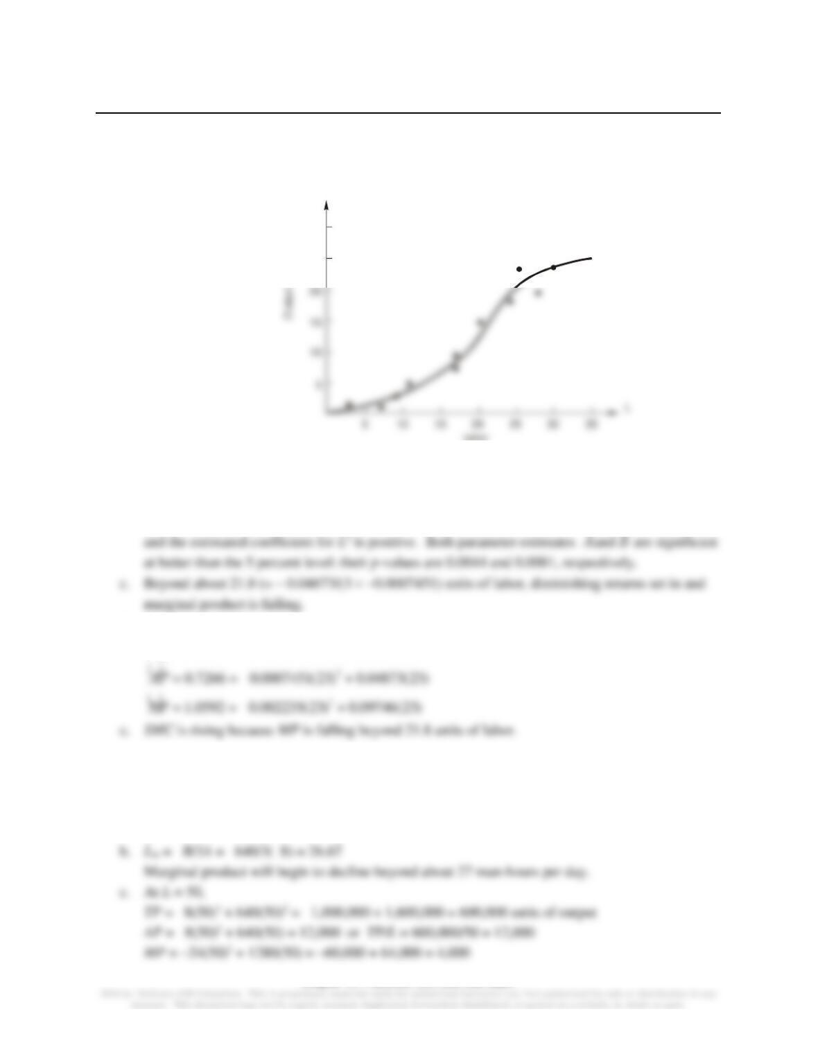
1. a. The scatter diagram for these data (shown below) strongly suggest a TP curve with an S-shape.
This scatter resembles the one shown in Figure 10.2 of the text. Thus, a cubic specification seems
most appropriate for these data.
Labor
TP
TP
25
30
b. The estimated short-run cubic production function is
ˆ
Q= –0.0007451L3+0.04873L2
The parameter estimates have the appropriate signs: the estimated coefficient for L3 is negative
d. At 23 units of labor:
ˆ
Q=16.71 = –0.0007451(23)3+0.04873(23)2
2. a. TP = –0.015625 (8)3 L3 + 10 (8)2 L2
= –8L3 + 640L2
AP = –8L2 + 640L
MP = –24L2 + 1280L
Chapter 10: Production and Cost Estimation
3. a. Only
ˆ
a
and
ˆ
b
are significant at the 2 percent level.
ˆ
c
is significant at the 2.62 percent level.
Answers to Mathematical Exercises
1. In order to have MP rise then fall, the slope of MP (MPLL) must first be positive at low levels of labor
usage and then negative at higher levels of labor usage. Since MPLL = 6AL + 2B, letting A > 0 and B
2.
Lm(K)= – bK 2
aK3= – b
aK–1
. Taking the derivative of Lm with respect to
K
, we see that this derivative
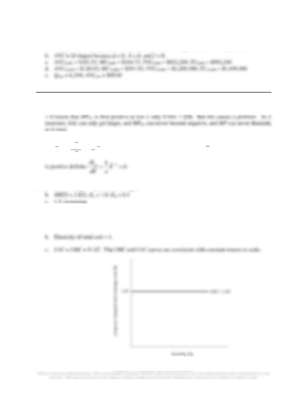
3. a. MPL = 1.0 Q/L and MPK = 0.5 Q/K
c. 1.5; increasing
4. a. Yes, because the exponents on w and r sum to one. Thus, LTC (Q; 2w, 2r) = 1/12 Q (2w)0.5(2r)0.5
= 2LTC(Q; w, r).