Head loss
Final calculations
121
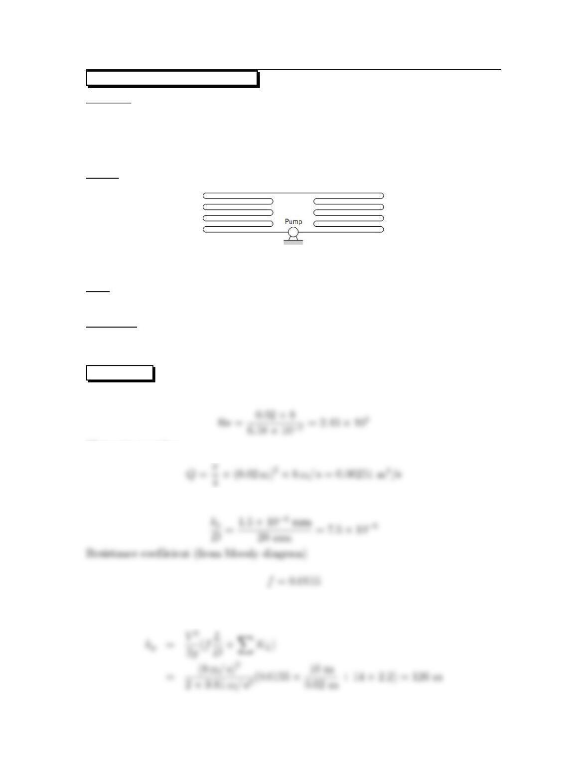
10.75: PROBLEM DEFINITION
Situation:
A heat exchanger is described in the problem statement.
V=8m/s,D=2cm.
η=0.85,L=10m.
14 – 180 ◦elbows, KL=2.2.
Sketch:
Find:
Power required to operate pump.
Properties:
Water (40 ◦C), Table A.5: ν=6.58 ×10⁻⁷m2/s, γ=9732N/m3
From Table 10.4 ks=0.0015 mm.
SOLUTION
Reynolds number
Flow rate equation
Relative roughness (copper tubing)
Energy equation
122
Power equation
123
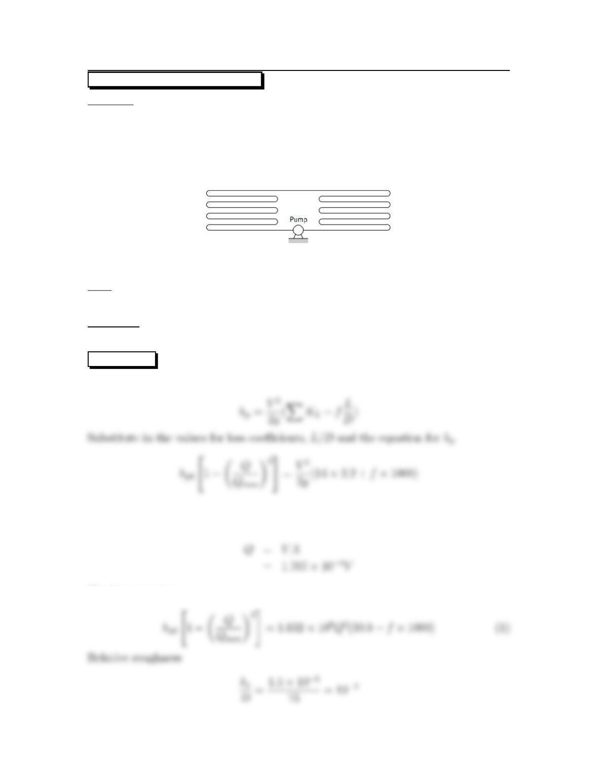
10.76: PROBLEM DEFINITION
Situation:
A heat exchanger is described in the problem statement.
L=15m,D=15mm.
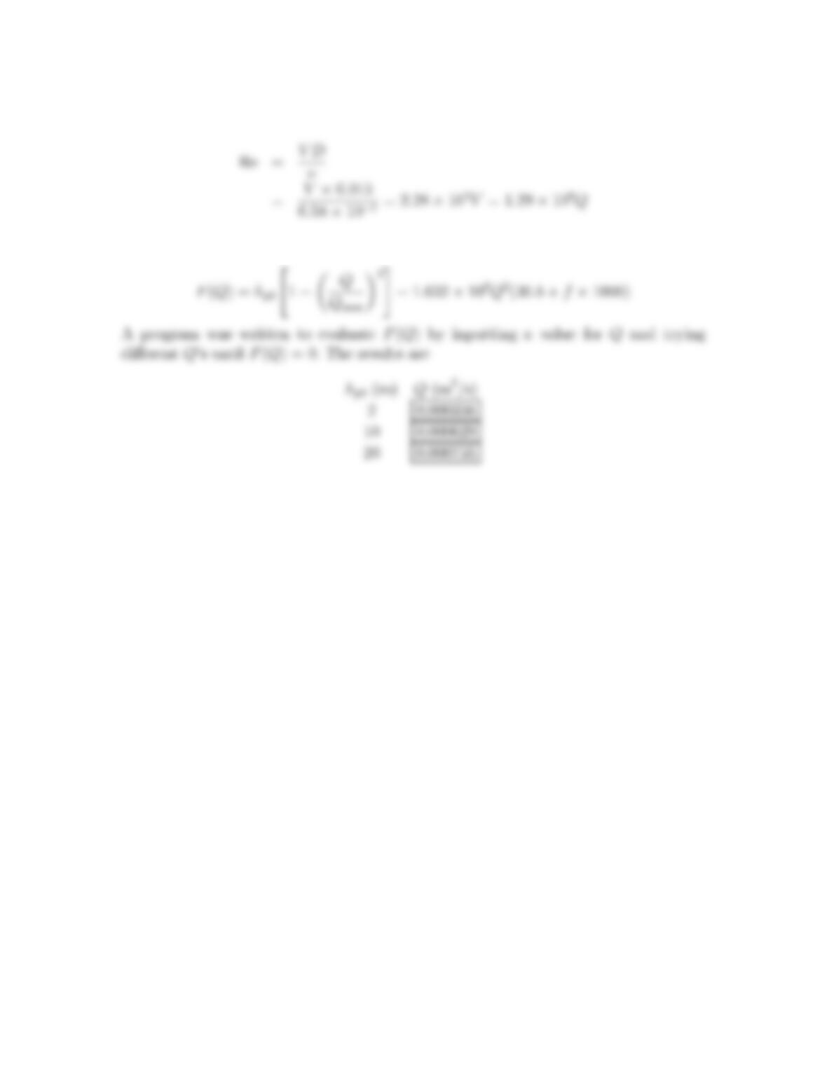
Qmax =10
−3m3/s.
hp=hp0[1 −(Q/Qmax)3].
14 – 180 ◦elbows, KL=2.2.
Find:
System operating points for hp0of 2m,10 m and 20 m.
Properties:
From Table 10.4: ks=1.5×10⁻³mm.
SOLUTION
Energy equation
Flow rate equation
Combine equations
124
Reynolds number
Eq. (1) becomes
125
10.77: PROBLEM DEFINITION
Situation:
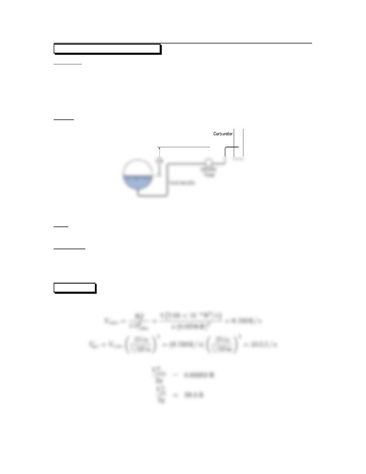
Gasoline being pumped from a gas tank.
Pressure in the tank = 14.7 psia, pressure in the carburetor = 14.0 psia.
Dtube =0.25 in = 0.0208 ft,Djet =1/32 in = 0.00260 ft.
L=10ft,
η=0.80,Q=0.12 gpm = 2.68 ×10⁻⁴cfs
Sketch:
Find:
Pump power.
Properties:
Gasoline Fig. A.2 (EFM10e): S=0.68,ν=5.5×10⁻⁶ft2/s, γ=62.4lbf/ft3×
0.68 = 42.4lbf/ft3
Loss coefficient, Table 10.5 (EFM10e), 90 ◦smooth bends, r/d =6,K
b=0.21.
SOLUTION
Velocity values
126
Reynolds number (fuel line)
From Moody diagram, Fig 10.14 (EFM10e)
f≈0.040
Energy equations
Power equation
127
10.78: PROBLEM DEFINITION
Situation:
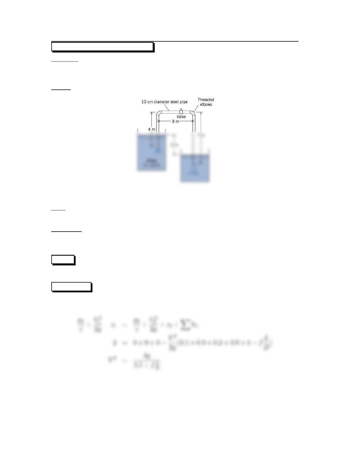
A partially-closed valve on a steel pipeline between two reservoirs.
D=10cm,∆z=2m,L=14m.
Sketch:
Find:
Loss coefficient for valve, Kv.
Properties:
From Table 10.4: ks=0.046 mm
Water (10 ◦C), Table A.5: v=1.31 ×10⁻⁶m2/s.
PLAN
First find Qfor valve wide open. Assume valve is a gate valve.
SOLUTION
Energy equation
128
Assume f=0.015.Then
From the Moody diagram, f=0.019.Then
This is close to 2.0×10⁵so no further iterations are necessary. For one-half the
discharge
129
10.79: PROBLEM DEFINITION
Situation:
A galvanized steel pipe connects a water main to a factory.
p1=350kPa,Q=0.025 m3/s.
L=160m,z2=8m,p2=70kPa.
Find:
Thepipesize.
Properties:
From Table 10.4 ks=0.15 mm.
Water (10 ◦C), Table A.5: γ=9810N/m3,ν=1.31 ×10−6m2/s.
SOLUTION
Energy equation
Assume f=0.020.Then
Relative roughness
130
Reynolds number
Friction factor (f)(Swamee-Jain correlation)
Recalculate pipe diameter
131
10.80: PROBLEM DEFINITION
Situation:
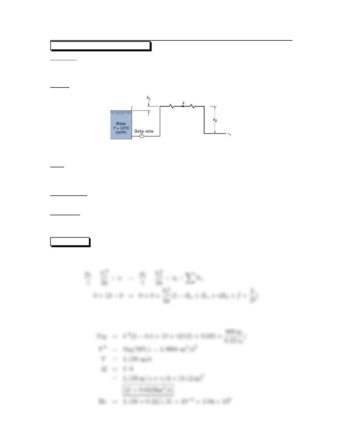
A steel pipe discharges into the atmosphere.
D=12cm,L=800m,z1=12m.
Sketch:
Find:
Discharge (m
3/s).
Pressure at point A.
Assumptions:
Water temperature is 10 ◦C.
Properties:
Water (10 ◦C),Table A.5: ν=1.31 ×10⁻⁶m2/s.
From Table 10.5: Kv=10,K
b=0.9,K
e=0.5.
SOLUTION
Energy equation
Using a pipe diameter of 10 cm and assuming f=0.025
132
From Fig. 10.8 f≈0.025
Note that this is not a good installation because the pressure at Ais near cavitation
level.
133
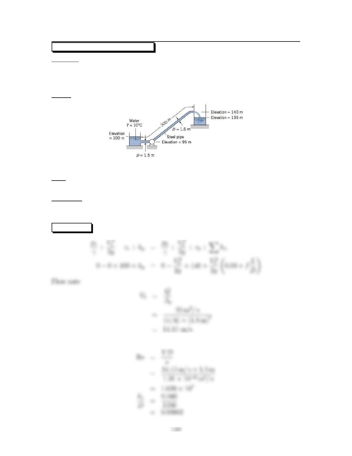
10.81: PROBLEM DEFINITION
Situation:
Water is pumped from one reservoir to another reservoir.
D=1.5m,Q=25m
3/s.
L=300m,z2=140m,z1=100m.
Sketch:
Find:
Pump power.
Properties:
From Table 10.4: ks=0.046 mm.
Water (10 ◦C),TableA.5ν=1.31 ×10⁻⁶mm.
SOLUTION Energy equation
Reynolds number
Friction factor (Moody Diagram) or the Swamee-Jain correlation:
Then
Power equation
135
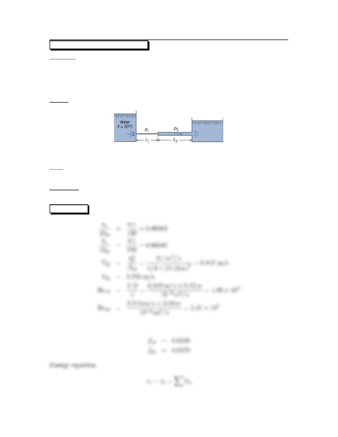
10.82: PROBLEM DEFINITION
Situation:
A system with two pipe sizes connects two reservoirs.
ks=0.1mm,Q=0.1m
3/s.
D1=12cm,L1=60m.
D2=24cm,L2=120m.
Sketch:
Find:
Difference in water surface between two reservoirs.
Properties:
Water (20oC), Table A.5: ν=10
−6m2/s.
SOLUTION
Resistance Coefficient (from the Moody diagram, Fig. 10-8)
136
137
10.83: PROBLEM DEFINITION
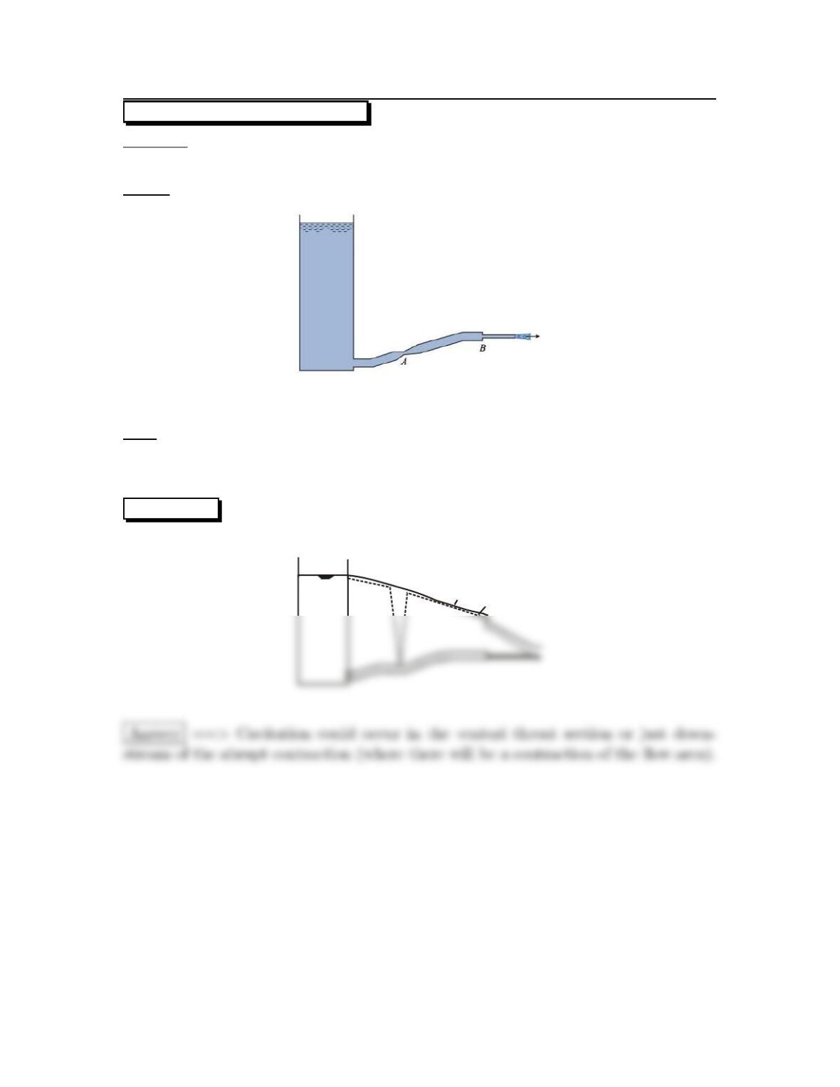
Situation:
A tank discharges to atmosphere through a piping system.
Sketch:
Find:
Sketch the EGL and HGL.
Identify where cavitation might occur.
SOLUTION
H.G
.L.
E.G
.L.
138
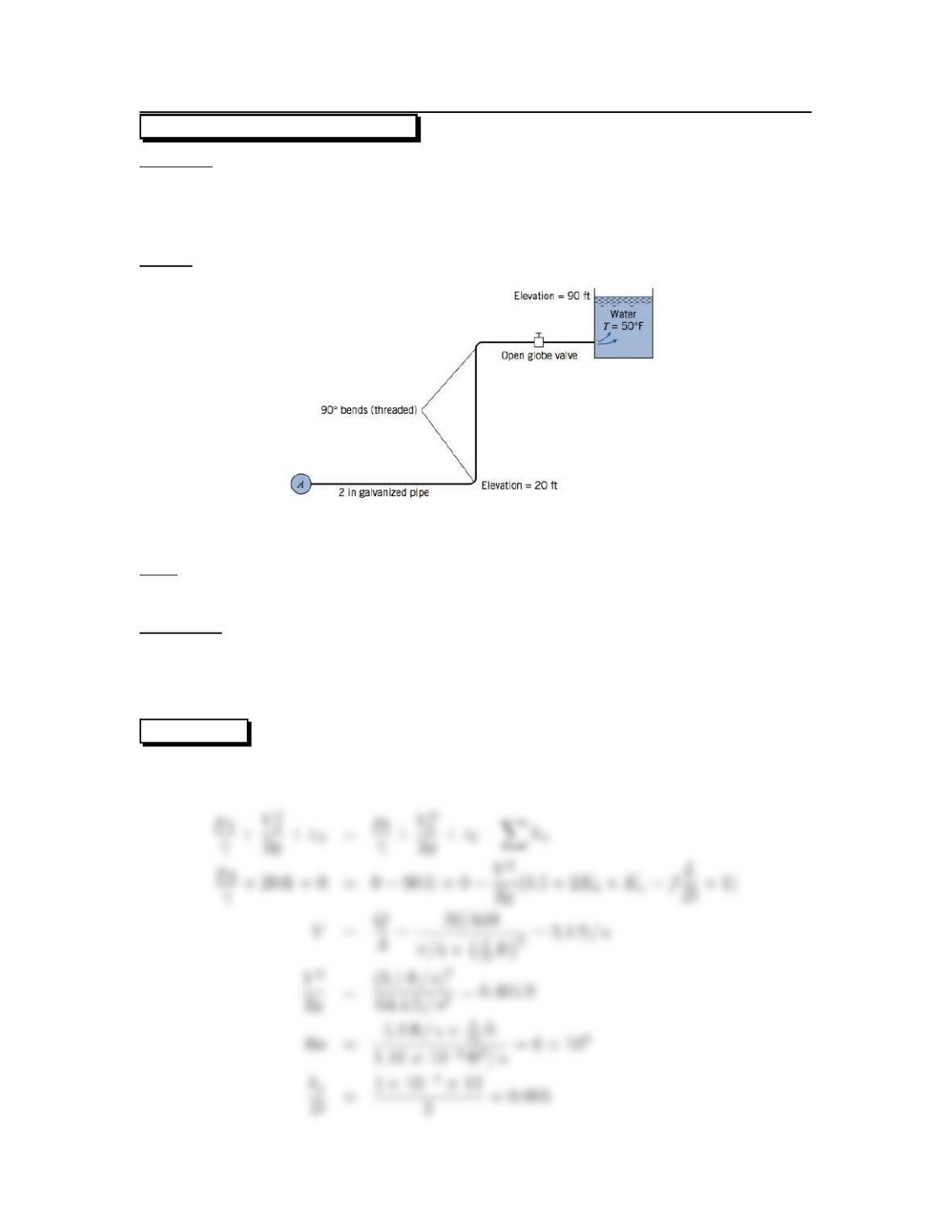
10.84: PROBLEM DEFINITION
Situation:
A steel pipe carries water from a main pipe to a reservoir.
z1=20ft,z2=90ft.
Q=50gpm, D=2in,L=240ft.
Sketch:
Find:
Pressure at point A.
Properties:
From Table 10.5: Kb=0.9,K
v=10.
From Table 10.4: ks=5×10⁻⁴ft.
Water (50 ◦F),TableA.5:ν=1.41 ×10⁻⁵ft2/s.
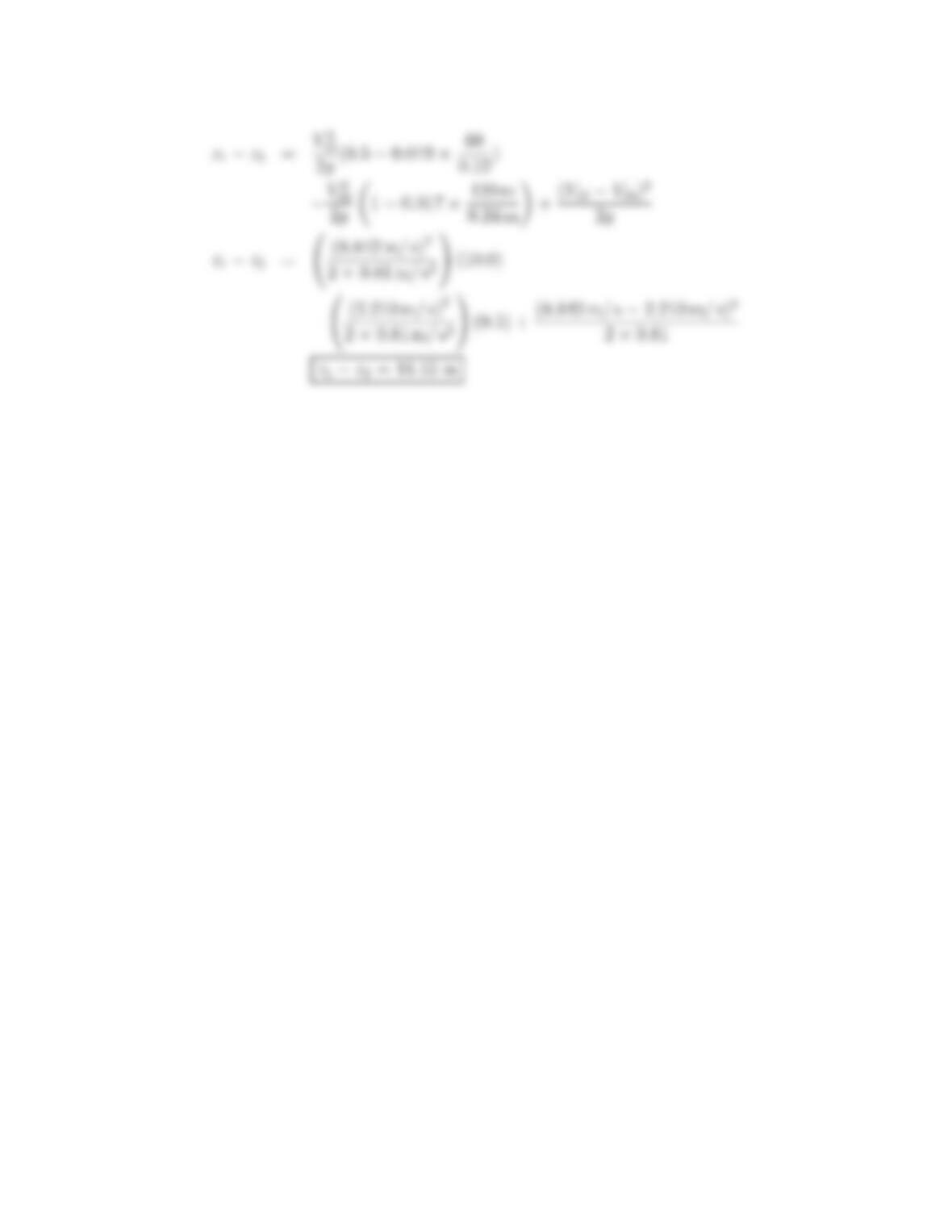
SOLUTION
Energy equation
139
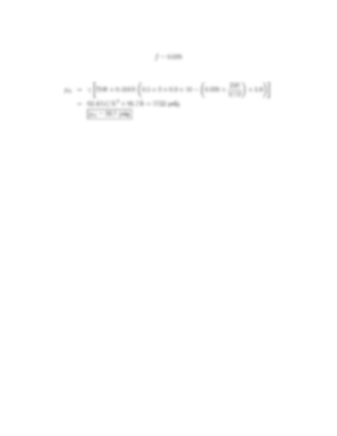
Resistance coefficient (from Moody diagram)
Energy equation becomes
140