CHAPTER 10 │ CHI-SQUARE TESTS AND THE
F
-DISTRIBUTION 437
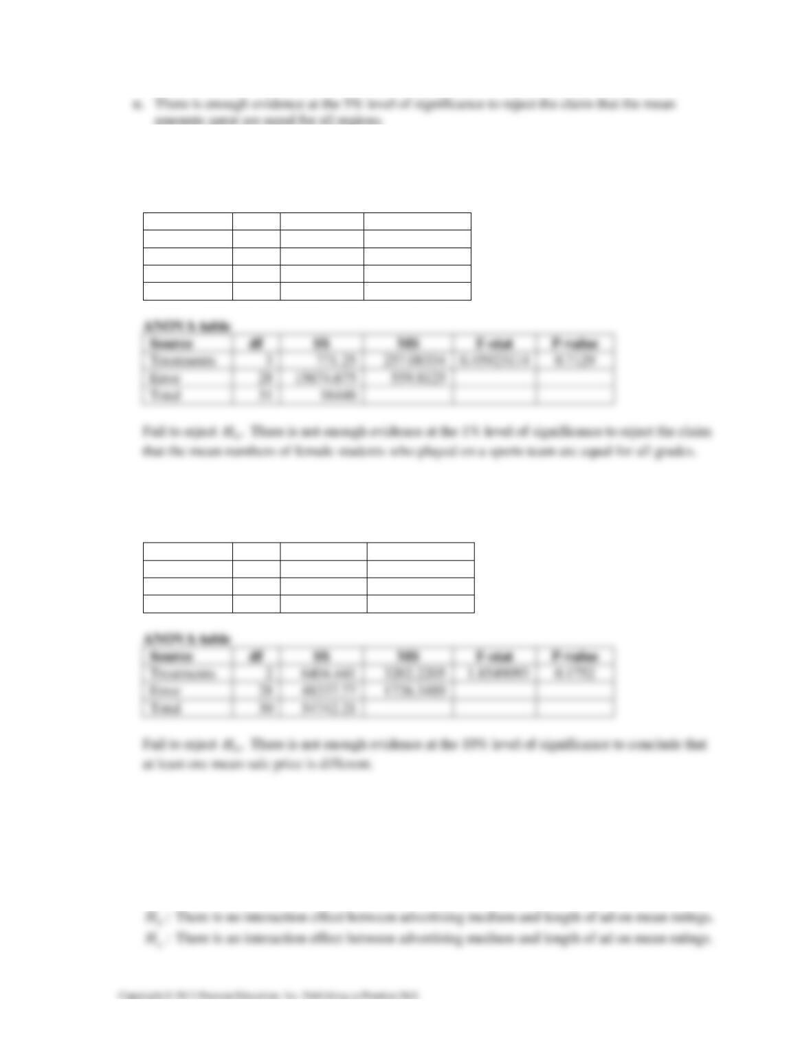
15. Analysis of Variance results:
Data stored in separate columns.
Column means
Column N Means Std. Error
Grade 9 8 84.375 9.531784
Grade 10 8 79.25 9.090321
Grade 11 8 76.625 7.648383
Grade 12 8 70.75 6.9224014
16. Analysis of Variance results:
Data stored in separate columns.
Column means
Column N Means Std. Error
Gainesville 11 188.67273 12.685002
Orlando 10 209.56 11.292428
Tampa 10 173.96 14.59111
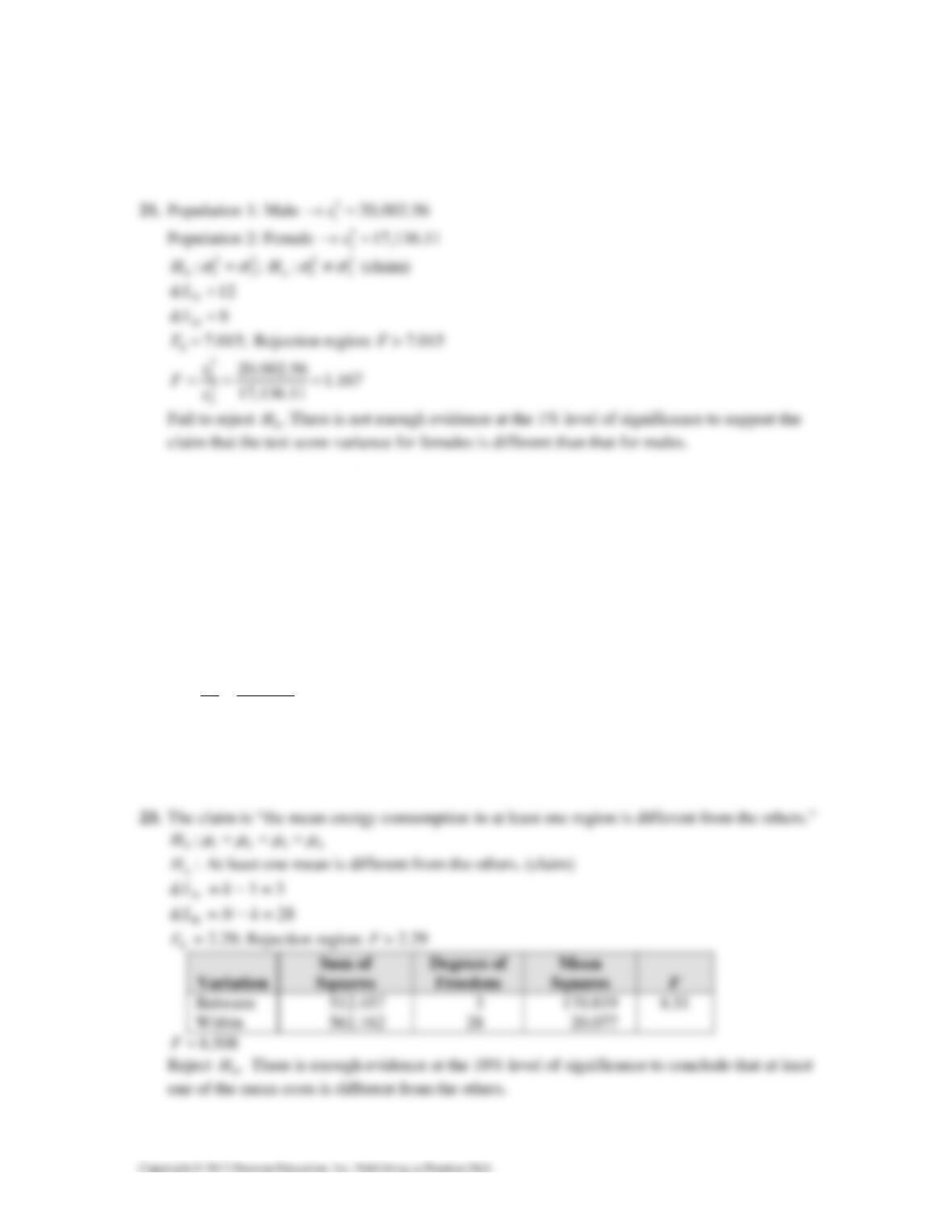
17. 0:H Advertising medium has to effect on mean ratings.
:
a
H Advertising medium has an effect on mean ratings.
0:H Length of ad has no effect on mean ratings.
:
a
H Length of ad has an effect on mean ratings.
438 CHAPTER 10 │ CHI-SQUARE TESTS AND THE
F
-DISTRIBUTION
18. 0:H Type of vehicle has no effect on the mean number of vehicles sold.
:
a
H Type of vehicle has an effect on the mean number of vehicles sold.
0:H Gender has no effect on the mean number of vehicles sold.
:
a
H Gender has an effect on the mean number of vehicles sold.
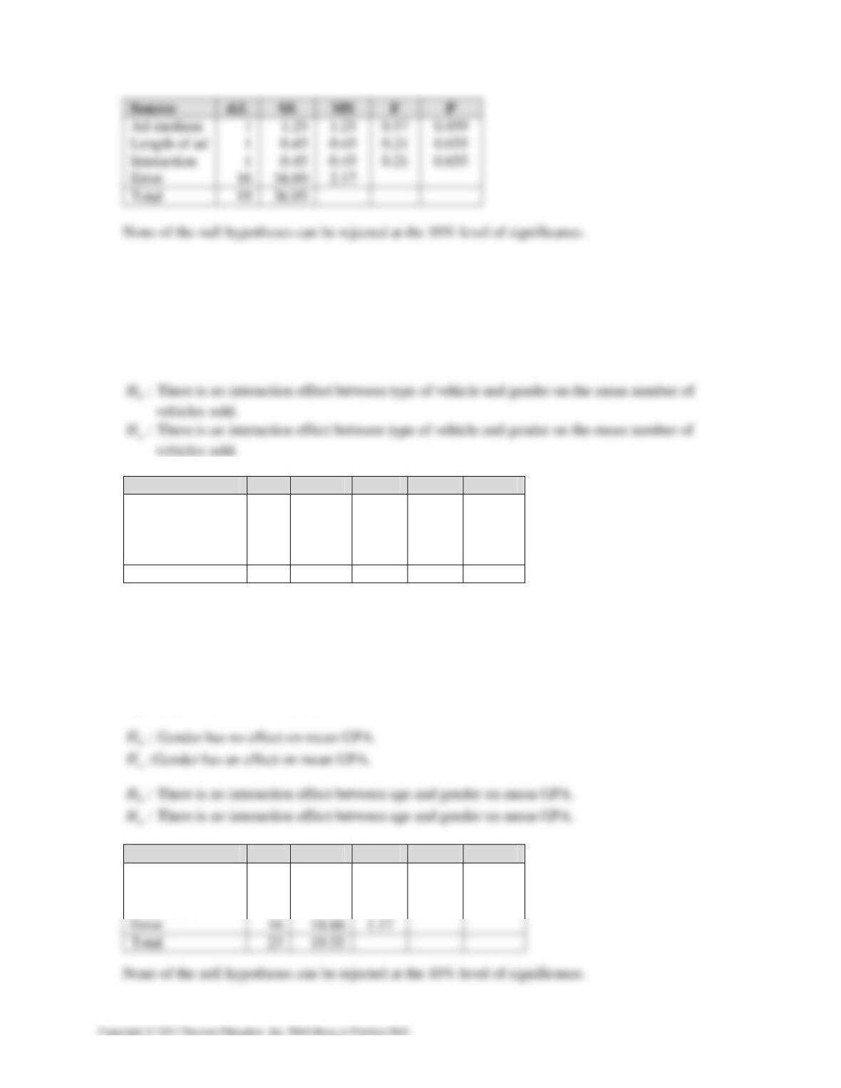
Source d.f. SS MS F P
Type of vehicle 2 84.08 42.04 34.01 0.000
Gender 1 0.38 0.38 0.30 0.589
Interaction 2 12.25 6.12 4.96 0.019
Error 18 22.25 1.24
Total 23 118.96
There appears to be an interaction effect between type of vehicle and gender on the mean number
of vehicles sold. Also, it appears that type of vehicle has an effect on the mean number of
vehicles sold.
19. 0:H Age has no effect on mean GPA.
:
a
H Age has an effect on mean GPA.
Source d.f. SS MS F P
Age 3 0.41 0.14 0.12 0.948
Gender 1 00.18 0.18 0.16 0.697
Interaction 3 0.29 0.10 0.08 0.968
CHAPTER 10 │ CHI-SQUARE TESTS AND THE
F
-DISTRIBUTION 439
20. 0:H Technicians have no effect on mean repair time.
:
a
H Technicians have an effect on mean repair time.
0:H Brand has no effect on mean repair time.
:
a
H Brand has an effect on mean repair time.
21.
Mean Size
Pop 1 66.36 10
Pop2 48.52 10
Pop3 42.27 10
1918.441
W
SS =
(1) 27
i
nNk−= −=
∑
0 Scheffe
5.49 CVF′
=→ = 5.49(3 − 1) = 10.98
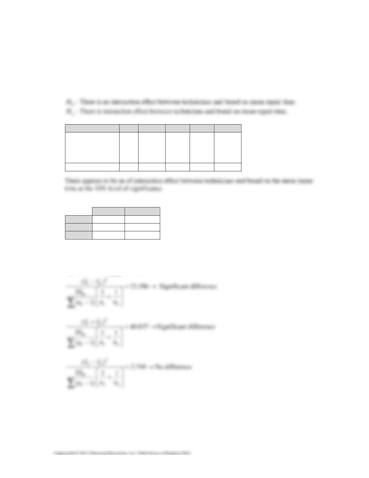
Source d.f. SS MS F P
Technicians 3 714 238 1.74 0.185
Brand 2 382 191 1.40 0.266
Interaction 6 2007 334 2.45 0.054
Error 24 3277 137
Total 35 6381
440 CHAPTER 10 │ CHI-SQUARE TESTS AND THE
F
-DISTRIBUTION
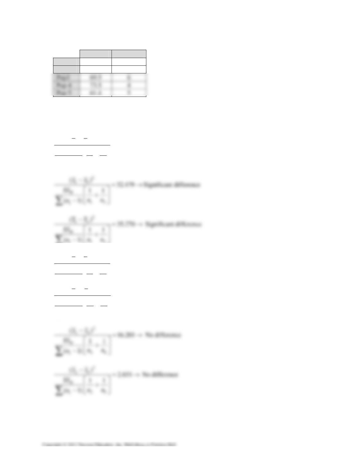
22.
Mean Size
Pop 1 43.6 5
Pop2 54.0 6
1182.900
W
SS =
(1) 21
i
nNk−= −=
∑
0 Scheffe
4.37 CVF′
=→ = 4.37(5 − 1) = 17.48
2
12
12
() 5.237
11
(1)
W
i
xx
SS
nn
n
−≈→
⎡⎤
+
⎢⎥
−⎣⎦
∑
No difference
i
∑
2
15
15
() 14.062
11
(1)
W
i
xx
SS
nn
n
−≈→
⎡⎤
+
⎢⎥
−⎣⎦
∑
No difference
2
23
23
() 12.795
11
(1)
W
i
xx
SS
nn
n
−≈→
⎡⎤
+
⎢⎥
−⎣⎦
∑
No difference
CHAPTER 10 │ CHI-SQUARE TESTS AND THE
F
-DISTRIBUTION 441
2
34
34
() 0.682
11
(1)
W
i
xx
SS
nn
n
−≈→
⎡⎤
+
⎢⎥
−⎣⎦
∑
No difference
23.
Mean Size
Pop 1 65.93 6
Pop2 66.1 8
Pop3 64.863 11
Pop 4 66.98 9
2
13
13
() 1.490
11
(1)
W
i
xx
SS
nn
n
−≈→
⎡⎤
+
⎢⎥
−⎣⎦
∑
No difference
2
14
14
() 1.345
11
(1)
W
i
xx
SS
nn
n
−≈→
⎡⎤
+
⎢⎥
−⎣⎦
∑
No difference
442 CHAPTER 10 │ CHI-SQUARE TESTS AND THE
F
-DISTRIBUTION
2
24
24
() 1.122
11
(1)
w
i
xx
SS
nn
n
−≈→
⎡⎤
+
⎢⎥
−⎣⎦
∑
No difference
24.
Mean Size
Pop 1 2312 10
Pop 2 1786 9
Pop 3 1755.142857 7
Pop 4 1491.285714 7
7, 017, 376.286
W
SS =
0 Scheffe
2.93 CVF′
=→ = 2.93(4 − 1) = 8.79
2
12
12
() 5.416
11
(1)
W
i
xx
SS
nn
n
−≈→
⎡⎤
+
⎢⎥
−⎣⎦
∑
No difference
2
14
14
() 11.462
11
(1)
W
i
xx
SS
nn
n
−≈→
⎡⎤
+
⎢⎥
−⎣⎦
∑
Significant difference
CHAPTER 10 │ CHI-SQUARE TESTS AND THE
F
-DISTRIBUTION 443
CHAPTER 10 REVIEW EXERCISE SOLUTIONS
1a.
Response Distribution
Less than $10 29%
b. 2
0
χ
= 6.251; Rejection region: 2
χ
> 6.251
c.
Response Distribution Observed Expected OE
E
2
()−
Less than $10 29% 353 319.87 3.431
$10 to $20 16% 167 176.48 0.509
4.886
24.886
χ
≈
d. Fail to reject 0.H
e. There is not enough evidence at the 10% level of significance to conclude that there has been a
change in the claimed or expected distribution.
2a.
χ
χ
Response Distribution
1−5 4%
6−10 24%
444 CHAPTER 10 │ CHI-SQUARE TESTS AND THE
F
-DISTRIBUTION
c.
Response Distribution Observed Expected OE
E
2
()−
1−5 4% 9 14 1.786
6−10 24% 62 84 5.762
213.809
χ
≈
d. Fail to reject 0.H
e. There is not enough evidence at the 1% level of significance to conclude that there has been a
change in the claimed or expected distribution.
3a.
0
c.
Response Distribution Observed Expected OE
E
2
()−
Short-game shots 65% 276 282.75 0.161
Approach and swing 22% 99 95.70 0.114
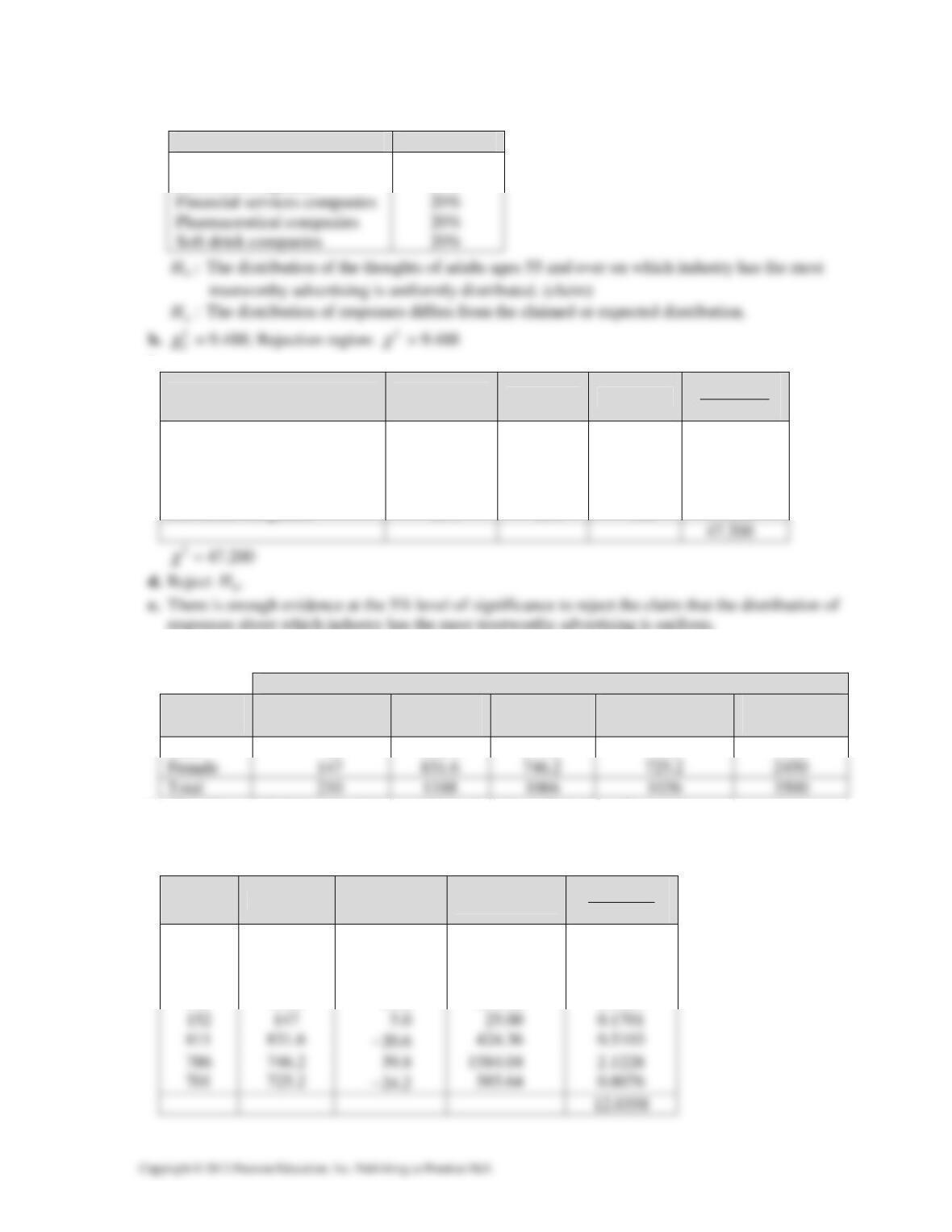
Response Distribution
Short-game shots 65%
Approach and swing 22%
Driver shots 9%
CHAPTER 10 │ CHI-SQUARE TESTS AND THE
F
-DISTRIBUTION 445
4a.
χ
χ
c.
Response Distribution Observed Expected OE
E
2
()−
Auto companies 20% 128 160 6.400
Fast food companies 20% 192 160 6.400
Financial services companies 20% 112 160 14.400
Pharmaceutical companies 20% 152 160 0.400
Soft drink companies 20% 216 160 19.600
responses about which industry has the most trustworthy advertising is uniform.
5a. Expected frequencies:
Years of full-time teaching experience
Gender
Less than
3 years
3−9 years
10−20 years
20 years
or more
Total
Male 63 356.4 319.8 310.8 1050
b. 0:H Years of full-time teaching experience is independent of gender.
:
a
H Years of full-time teaching experience is dependent on gender.
2
0
χ
= 11.345
O E O
−
E OE
2
()− OE
E
2
()
−
58 63.0 −5.0 25.00 0.3968
377 356.4 20.6 424.36 1.1907
280 319.8 −39.8 1584.04 4.9532
335 310.8 24.2 585.64 1.8843
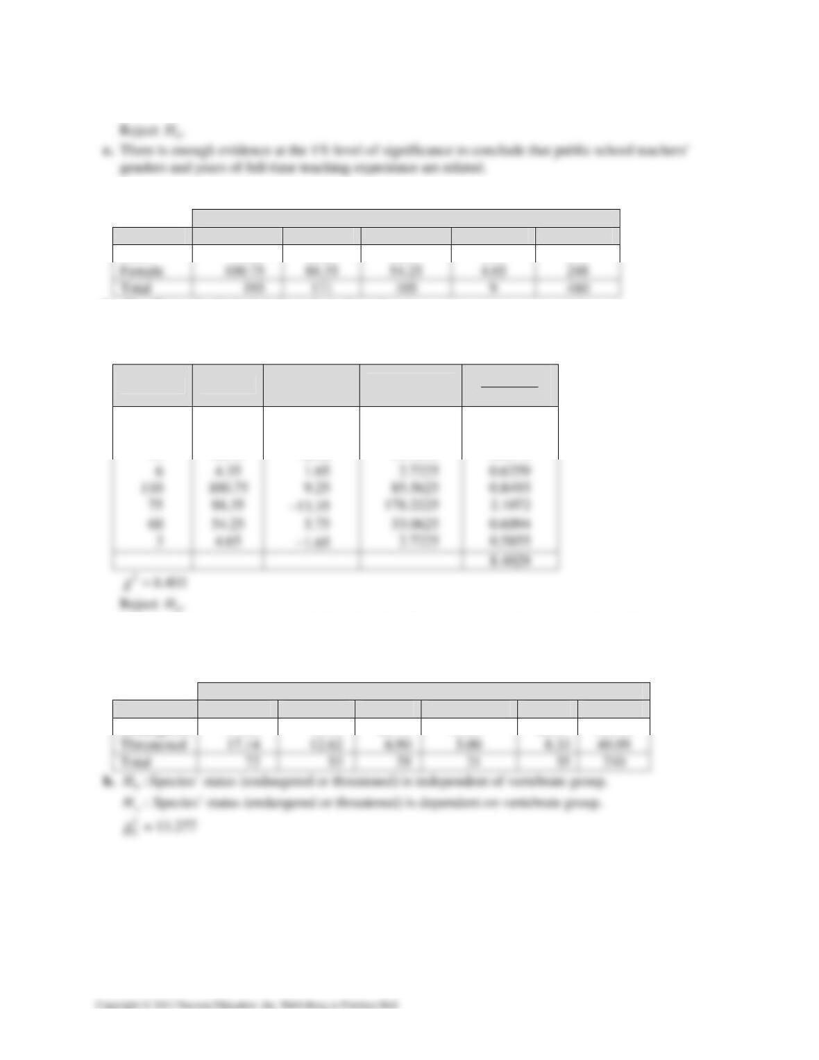
Response Distribution
Auto companies 20%
Fast food companies 20%
446 CHAPTER 10 │ CHI-SQUARE TESTS AND THE
F
-DISTRIBUTION
212.036
χ
≈
6a. Expected frequencies:
Type of vehicles owned
Gender Car Truck SUV Van Total
Male 94.25 82.65 50.75 4.35 232
b. 0:H Type of vehicle is independent of gender.
:
a
H Type of vehicle is dependent on gender.
2
0
χ
= 7.815
O E O
−
E OE
2
()− OE
E
2
()
−
85 94.25 −9.25 85.5625 0.9078
96 82.65 13.35 178.2225 2.1564
45 50.75 −5.75 33.0625 0.6515
0.H
c. There is enough evidence at the 5% level of significance to conclude that type of vehicle owned
is dependent on gender.
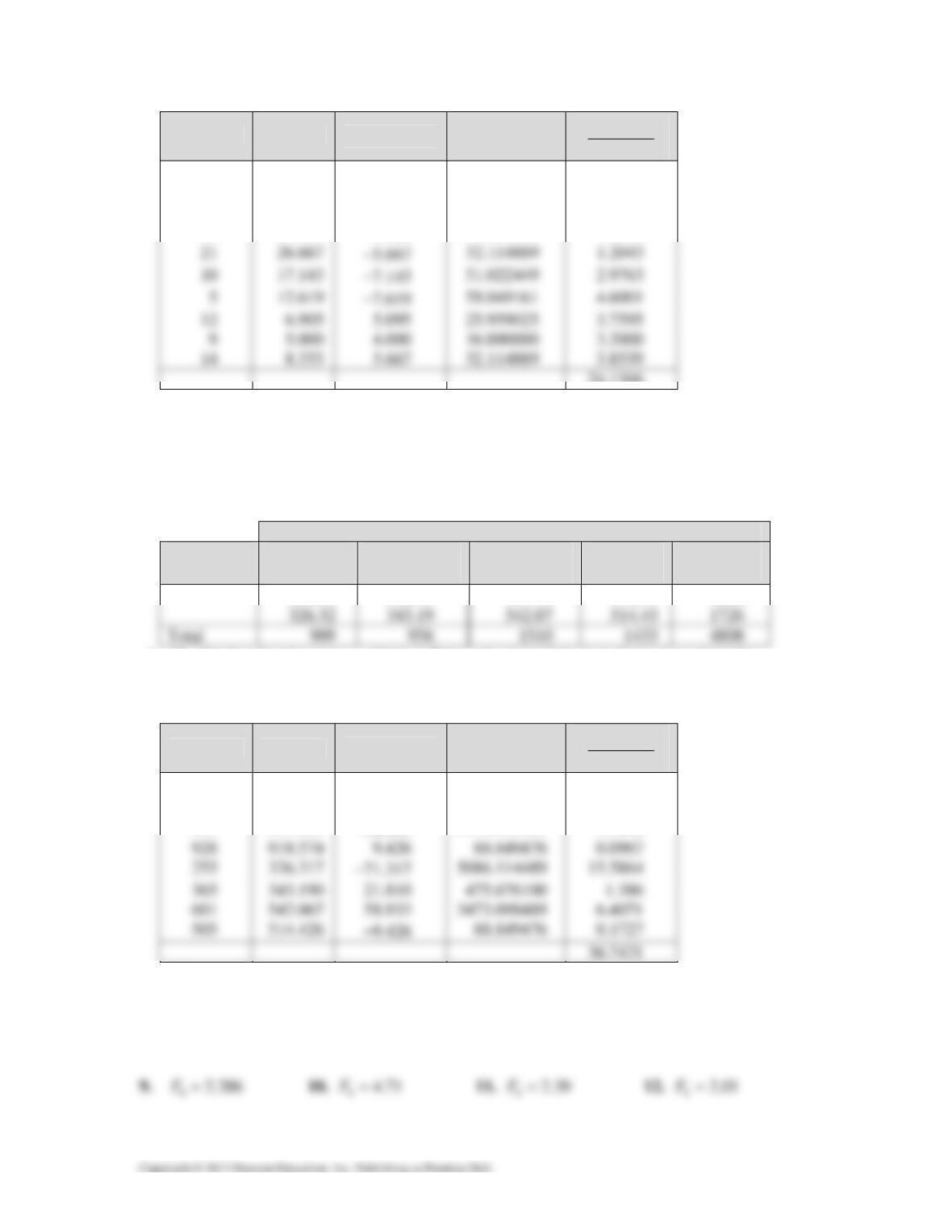
7a. Expected frequencies:
Vertebrae Group
Status Mammals Birds Reptiles Amphibians Fish Total
Endangered 54.86 40.38 22.10 16.00 26.67 160.01
χ
CHAPTER 10 │ CHI-SQUARE TESTS AND THE
F
-DISTRIBUTION 447
O E O
−
E OE
2
()− OE
E
2
()
−
62 54.857 7.143 51.022449 0.9301
48 40.381 7.619 58.049161 1.4375
17 22.095 5.095 25.959025 1.1749
12 16.000
−4.000 16.000000 1.0000
24.1366
224.154
χ
≈
Reject
0.H
c. There is enough evidence at the 1% level of significance to conclude that species’ status
(endangered or threatened) is dependent on vertebrate group.
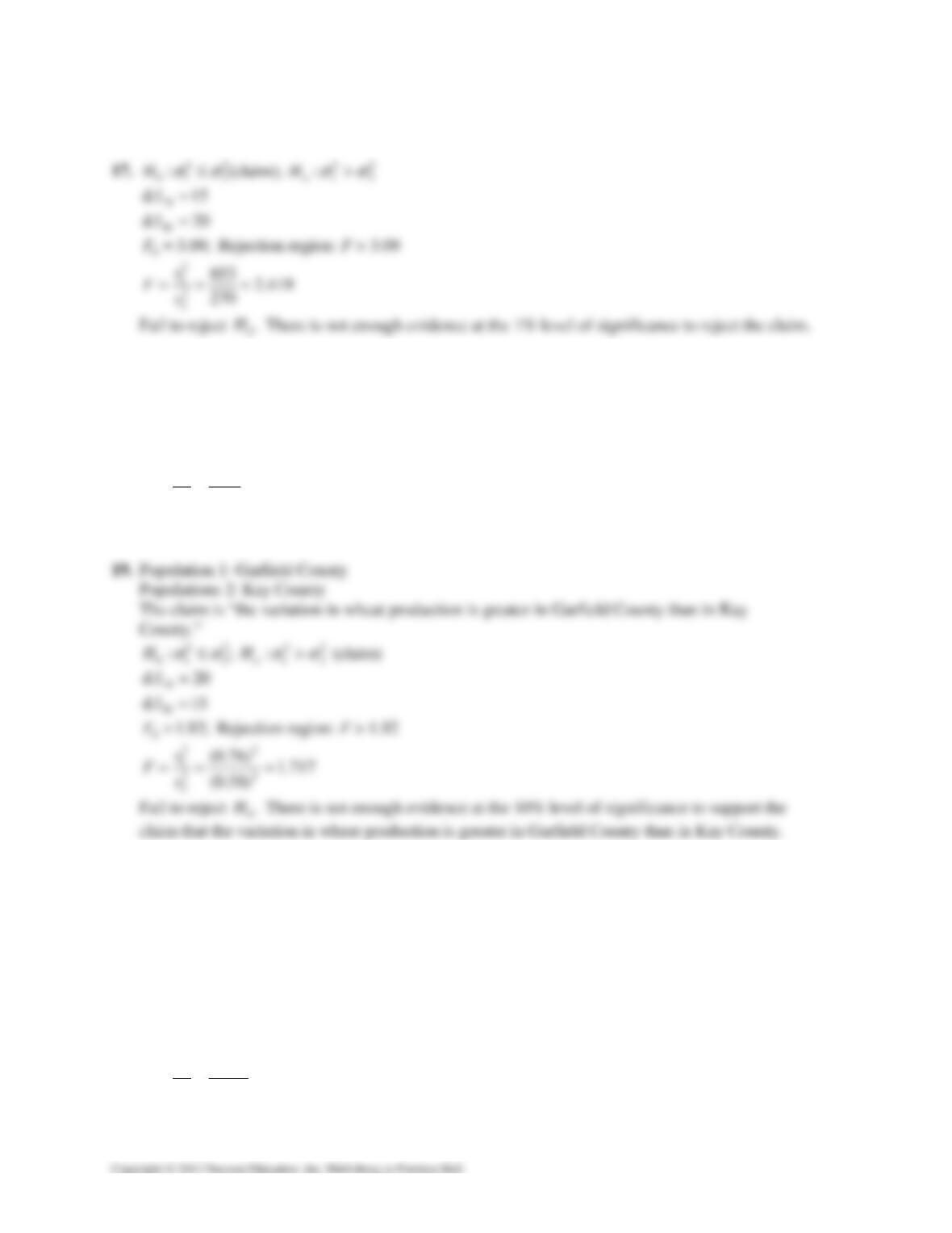
8a. Expected frequencies:
Time of day
Gender
12 AM−
5:59 AM
6 AM−
11:59 AM
12 PM−
5:59 PM
6 PM −
11:59 PM
Total
582.68 612.81 967.93 918.57 3082
b. 0:HFatal pedestrian motor vehicle collisions by time of day is independent of gender.
:
a
H Fatal pedestrian motor vehicle collisions by time of day is dependent on gender..
2
0
χ
= 6.251
O E O
−
E OE
2
()− OE
E
2
()
−
654 582.683 71.317 5086.114489 8.7289
591 612.810
−21.810 475.676100 0.7762
909 967.933
−58.933 3473.098489 3.5882
236.742
χ
≈
Reject
0.H
c. There is enough evidence at the 10% level of significance to conclude that the time of day of a
collision is dependent on gender.
448 CHAPTER 10 │ CHI-SQUARE TESTS AND THE
F
-DISTRIBUTION
13. 02.06F≈ 14. 04.36F= 15. 02.08F= 16. 04.73F=
18. 22 22
01 2 1 2
:; : (claim)
a
HH
σσ σσ
=≠
N
d.f. 30=
D
d.f. 28=
01.87;F= Rejection region: F > 1.87
2
1
2
2
87.3 1.919
45.5
s
F
s
== ≈
Reject
0.H There is enough evidence at the 10% level of significance to support the claim.
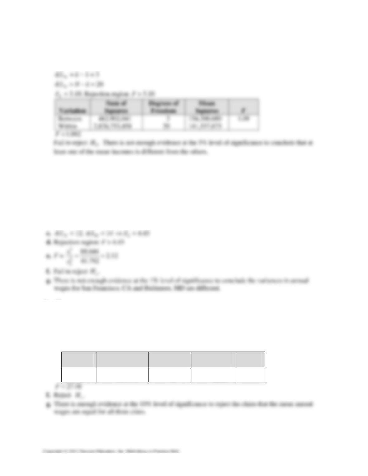
20. Population 1: San Francisco 1$44s→=
Population 2: Sacramento 2$44s→=
The claim is “the standard deviations of hotel rooms rates for San Francisco. (A and Sacramento,
CA are the same.”
22 22
01 2 1 2
: (claim); :
a
HH
σσ σσ
=≠
N
d.f. 35=
D
d.f. 30=
02.569;F= Rejection region: F >2.569
22
1
22
2
(75) 2.905
(44)
s
F
s
== ≈
CHAPTER 10 │ CHI-SQUARE TESTS AND THE
F
-DISTRIBUTION 449
Reject
0.H
There is enough evidence at the 1% level of significance to reject the claim that the standard
deviations of hotel room rates for San Francisco, CA and Sacramento, CA are the same.
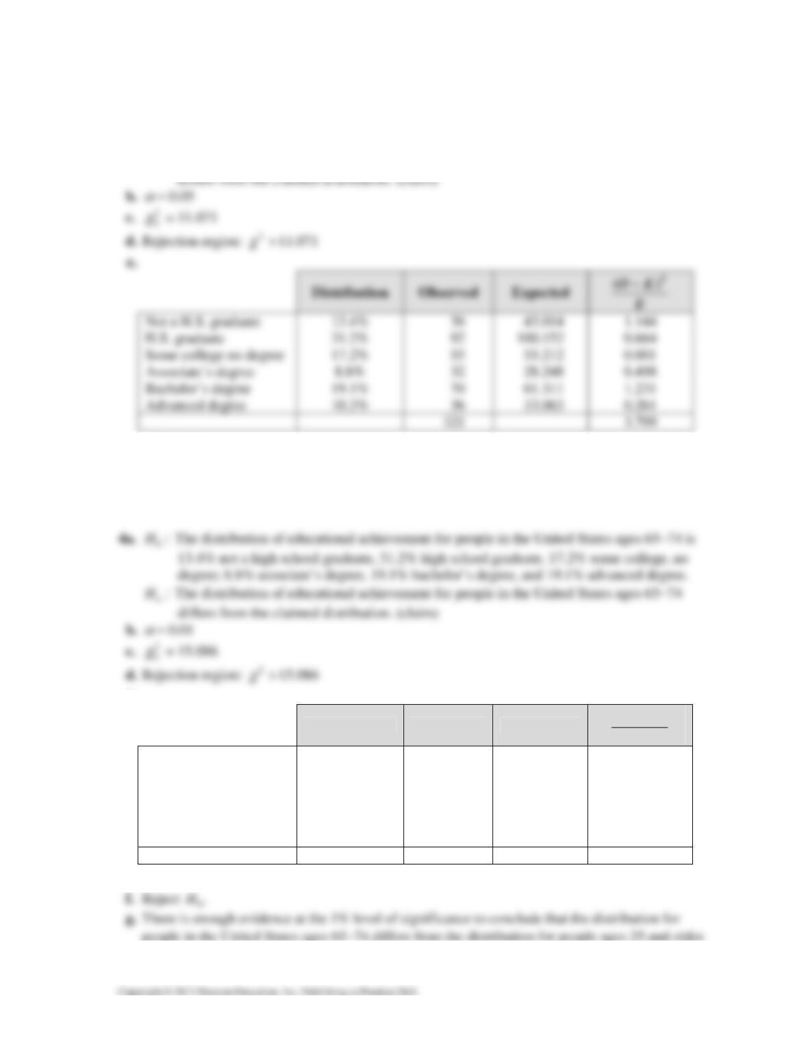
22. Population 1: Current 2
10.00146s→=
Population 2: New 2
20.00050s→=
The claim is “the new mold produces inserts that are less variable in diameter than the inserts the
current mold produces.”
22 22
01 2 1 2
:; : (claim)
a
HH
σσ σσ
≤> 22 22
01 2 1 2
:; : (claim)
a
HH
σσ σσ
≤>
N
d.f. 11=
D
d.f. 11=
02.82;F= Rejection region: F > 2.82
2
1
2
2
0.00146 2.92
0.00050
s
F
s
== ≈
Reject
0.HThere is enough evidence at the 5% level of significance to support the claim that the
new mold produces inserts that are less variable in diameter than the inserts the current mold
produces.
450 CHAPTER 10 │ CHI-SQUARE TESTS AND THE
F
-DISTRIBUTION
24. The claim is “at least one of the mean incomes is different from the others.”
01234
:H
µ
µµµ
===
:
a
H At least one mean is different from the others. (claim)
CHAPTER 10 QUIZ SOLUTIONS
1. Population 1: San Francisco 2
188.664s→=
Population 2: Baltimore 2
241.792s→=
a. 22 22
01 2 1 2
:; : (claim)
a
HH
σσ σσ
=≠
b. 0.01
α
=
2a. 01234
:H
µ
µµµ
===
:
a
H At least one mean is different from the others. (claim)
b. 0.10
α
=
c. N
d.f. = 2, D
d.f. = 40 0
F⇒ = 2.44
d. Rejection region: F > 2.44
e.
Variation
Sum of
Squares
Degrees of
Freedom
Mean
Squares
F
Between 3423.12 2 1711.56 27.48
Within 2491.79 40 62.29
CHAPTER 10 │ CHI-SQUARE TESTS AND THE
F
-DISTRIBUTION 451
3a. 0:H The distribution of educational achievement for people in the United States ages 35−44 is
13.4% not a high school graduate, 31.2% high school graduate, 17.2% some college, no
degree; 8.8% associate’s degree, 19.1% bachelor’s degree, and 10.3% advanced degree.
:
a
H The distribution of educational achievement for people in the United States ages 35−44
23.799
χ
≈
f. Fail to reject 0.H
g. There is not enough evidence at the 5% level of significance to conclude that the distribution for
people in the United States ages 35−44 differs from the distribution for ages 25 and older.
e.
Distribution Observed Expected OE
E
2
()
−
Not a H.S. graduate 13.4% 86 60.434 10.8154
H.S. graduate 31.2% 161 140.712 2.9251
Some college no degree 17.2% 72 77.572 0.4002
Associate’s degree 8.8% 27 39.688 4.0563
Bachelor’s degree 19.1% 60 86.141 7.9329
Advanced degree 10.3% 45 46.453 0.0454
451 26.175
226.175
χ
≈