Stress Distribution and Settlement Analysis Chapter 10
CHAPTER 10
STRESS DISTRIBUTION AND SETTLEMENT ANALYSIS
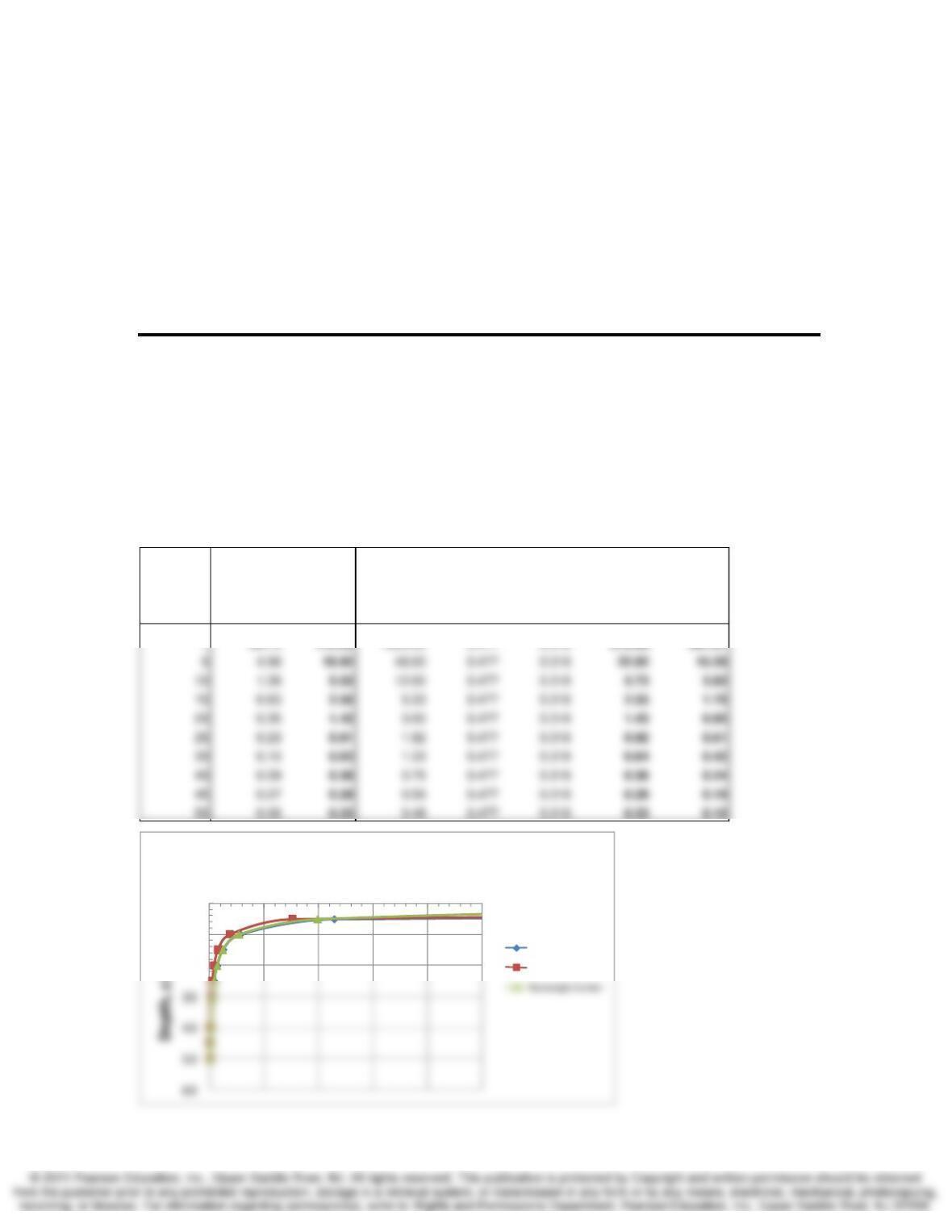
10-1. Compare the stress distribution with depth for (a) a point load of 1200 kN and (b) a 1200
kN load applied over an area of 3 x3 m. Plot the results.
10-2. If you used the Boussinesq (or Westergaard) theory for Problem 10.1, do the problem
again but use the Westergaard (or Boussinesq) theory instead. Comment on the differences
between the two theories.
SOLUTION:
Corner Center
Depth, z σ
z
4σ
z
Q/z
2
N
Bouss
N
west
σ
z
– Bouss σ
z
– West
(m) (kPa) (kPa) (kPa) (kPa) (kPa)
1 28.76 115.02 1200.00 0.477 0.318 572.96 381.97
Rectangular Load Point Load
0
10
20
0 1020304050
StressIncrease(kPa)
Boussinesq
Westergaard
Stress Distribution and Settlement Analysis Chapter 10
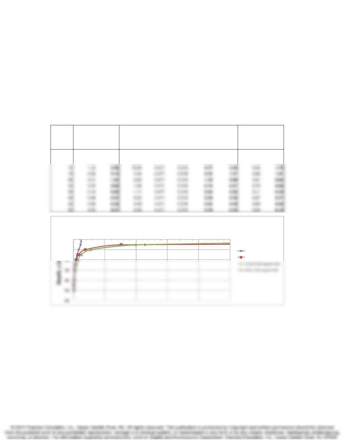
10-3. Compute the data and draw a curve of
σ
z/Q versus depth for points directly below a point
load Q. On the same plot draw curves of
σ
z/Q versus depth for points directly below the center of
square footings with breadths of 6.5 m and 20 m, respectively, each carrying a uniformly
distributed load Q. On the basis of this plot, make a statement relative to the range within which
loaded areas may be considered to act as point loads. (After Taylor, 1948.)
SOLUTION:
As can be viewed in the plot, at a depth of about two times the loaded area, the σz value is not
significantly different than the point load solution. (A Q value of 1000 was used in this solution.)
Corner Center Corner Center
Depth, z σz4σzQ/z2NBouss Nwest σz – Bouss σz – West σz4σz
(m) (kPa) (kPa) (kPa) (kPa) (kPa) (kPa) (kPa)
16.2825.10 1000.00 0.477 0.318 477.46 318.31 0.62 2.50
53.0112.04 40.00 0.477 0.318 19.10 12.73 0.58 2.32
6.5 m x 6.5 m Load Point Load 20 m x 20 m Load
0
10
0 1020304050
StressIncrease(kPa)
Boussinesq
Westergaard
Stress Distribution and Settlement Analysis Chapter 10
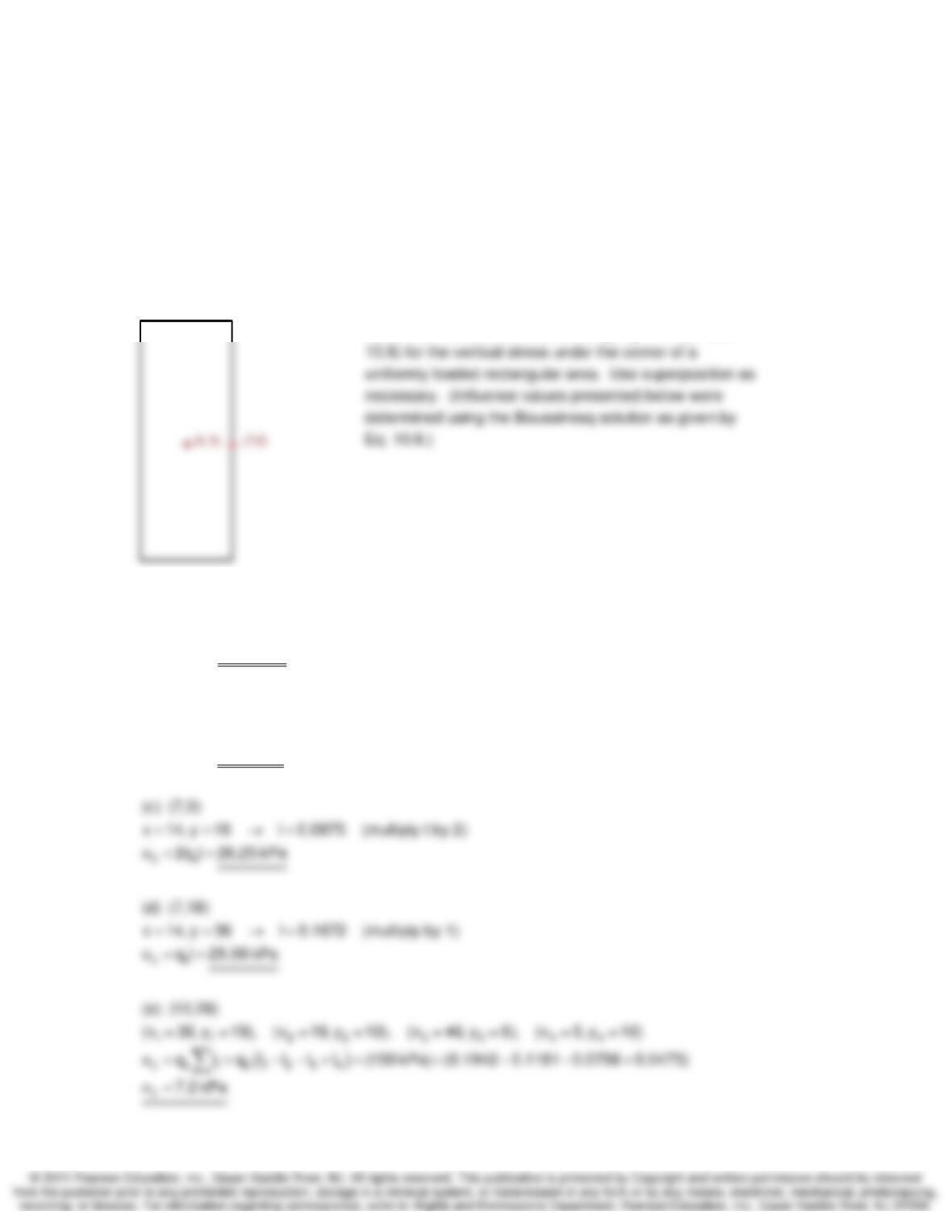
10-4. The center of a rectangular area at ground surface has Cartesian coordinates (0, 0), and
the corners have coordinates (7, 18). All dimensions are in meters. The area carries a uniform
pressure of 150 kPa. Estimate the stresses at a depth of 20 m below ground surface at each of
the following locations using the Boussinesq approach: (0, 0), (0, 18), (7, 0), (7, 18), and (12, 28).
SOLUTION:
(7, 18)
+
(0, 18)
+(12,28)
zo
zo
(a) (0,0)
x 7, y 9 I 0.0592 (multiply I by 4)
4q I 35.49 kPa
(b) (0,18)
x 7, y 36 I 0.1007 (multiply I by 2)
2q I 30.21kPa
==→=
σ= =
== →=
σ= =
qo = 150 kPa and z = 20 m
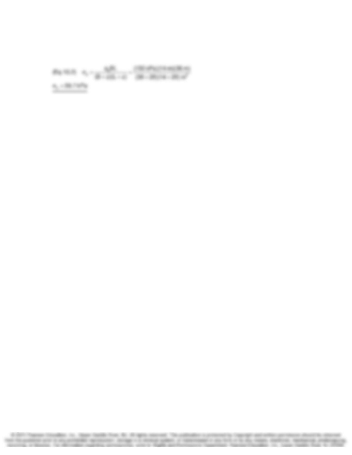
Determine the stress increase using Fig. 10.4 (or Eq.
Stress Distribution and Settlement Analysis Chapter 10
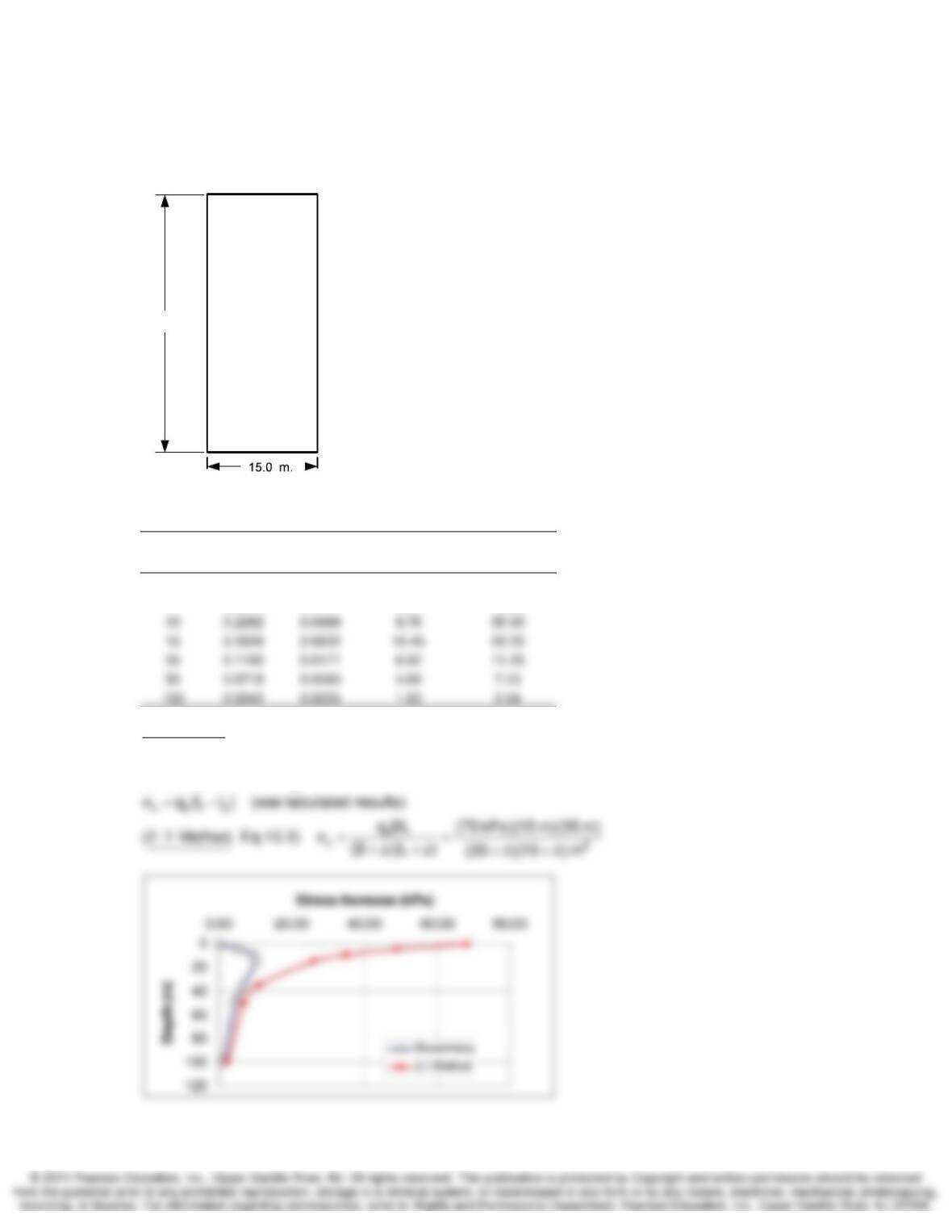
10-5. Compare the results of Problem 10.4 with those of the 2:1 method. Comments?
SOLUTION:
Stress Distribution and Settlement Analysis Chapter 10
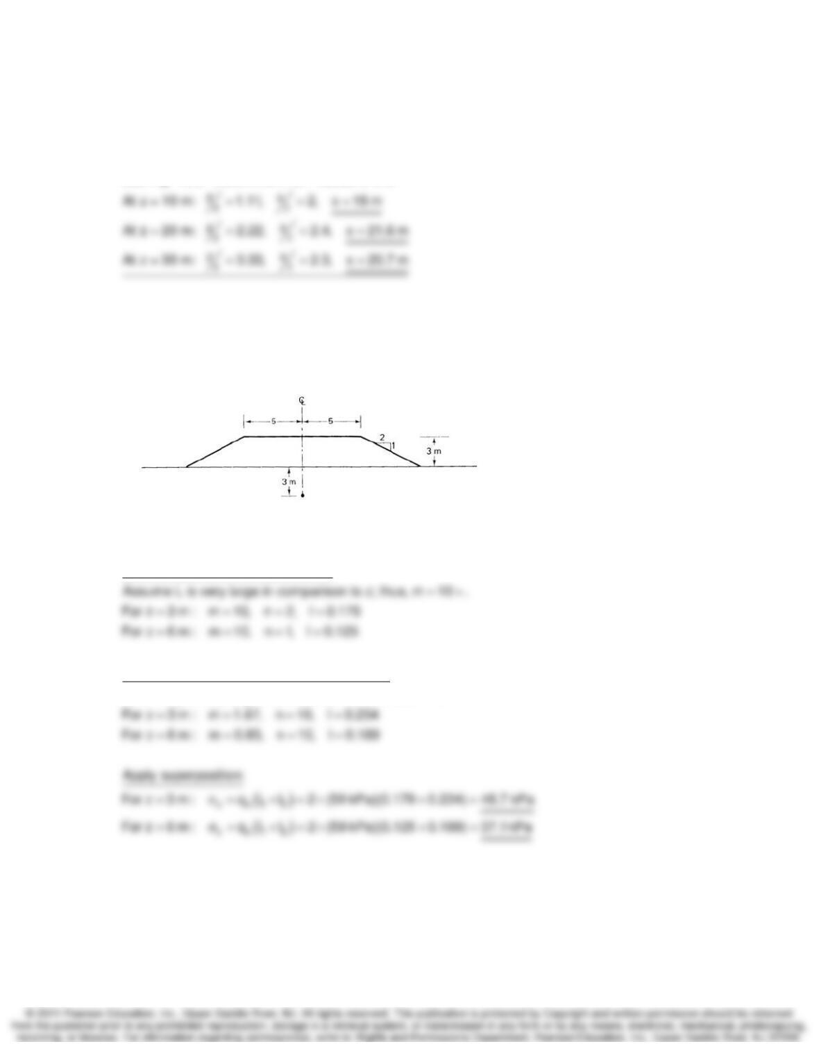
10-6. Calculate the stress distribution with depth at a point 3.5 m from the corner (along the
longest side) of a rectangularly loaded area 15 by 35 m with a uniform load of 75 kPa.
+
(
0, 0
)
(15, 38.5)
+
35.0 m.
SOLUTION:
Boussinesq 2:1 Method
Depth Ι
1
Ι
2
Δσ
v
Δσ
v
(m) (kPa) (kPa)
1 0.2500 0.2477 0.17 68.36
5 0.2464 0.1711 5.65 49.22
1
2
Bous sin esq
x38.5,y15 I
x3.5,y15 I
==→
==→
qo = 75 kPa and z varies
Determine the stress increase using Fig. 10.4 (or Eq.
10.6) for the vertical stress under the corner of a
uniformly loaded rectangular area. Use superposition as
necessary. (Influence values presented below were
determined using the Boussinesq solution as given by
Eq. 10.6.)
Stress Distribution and Settlement Analysis Chapter 10
10-7. How far apart must two 18 m diameter tanks be placed such that their stress overlap is not
greater than 10% of the contact stress at depths of 10, 20, and 30 m?
SOLUTION:
Use Fig. 10.5. Determine x for I values of 5%
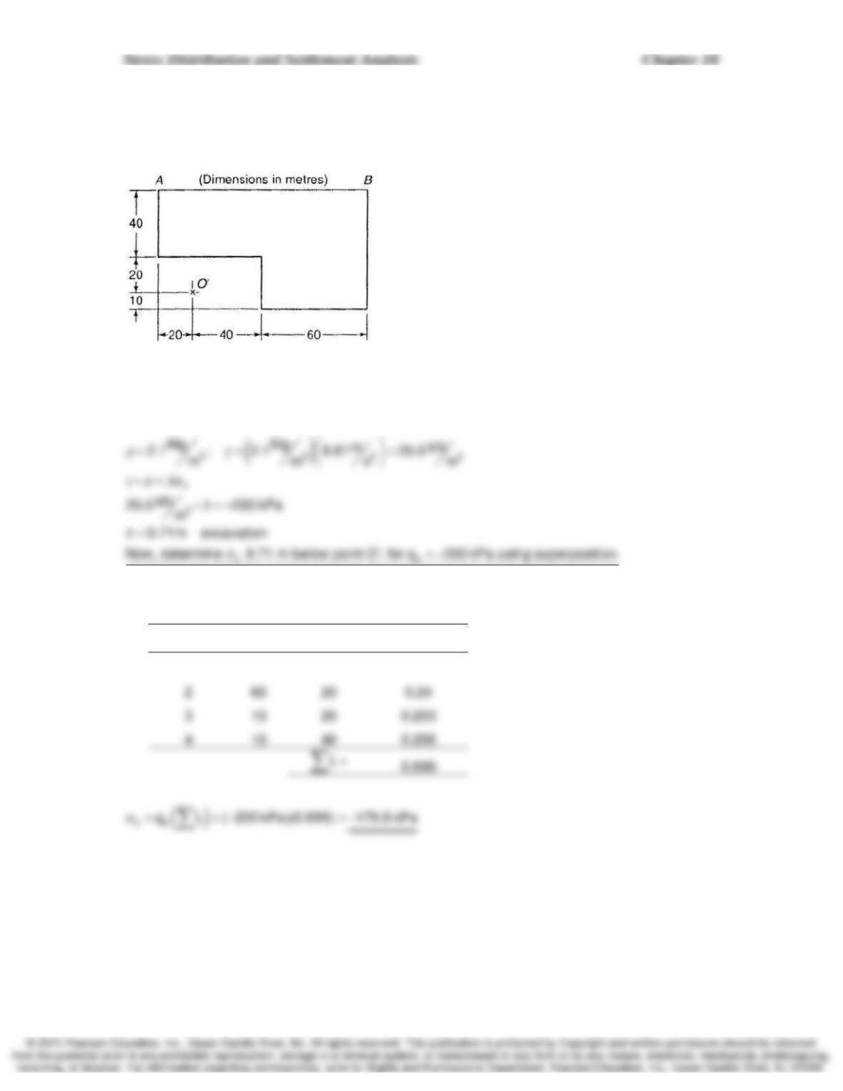
10-9. Work Example 10.5, using superposition of the results of Figs. 10.7 and 10.4. How does
your answer compare with the solution for Example 10.5?
SOLUTION:
Scan fig from p.471
−
−
Fig. 10.7 Corner of triangular load:
Fig. 10.4 Corner of rectangular loaded area:
Assume y is very la
=+
rge in comparison to x; thus, n 10 .
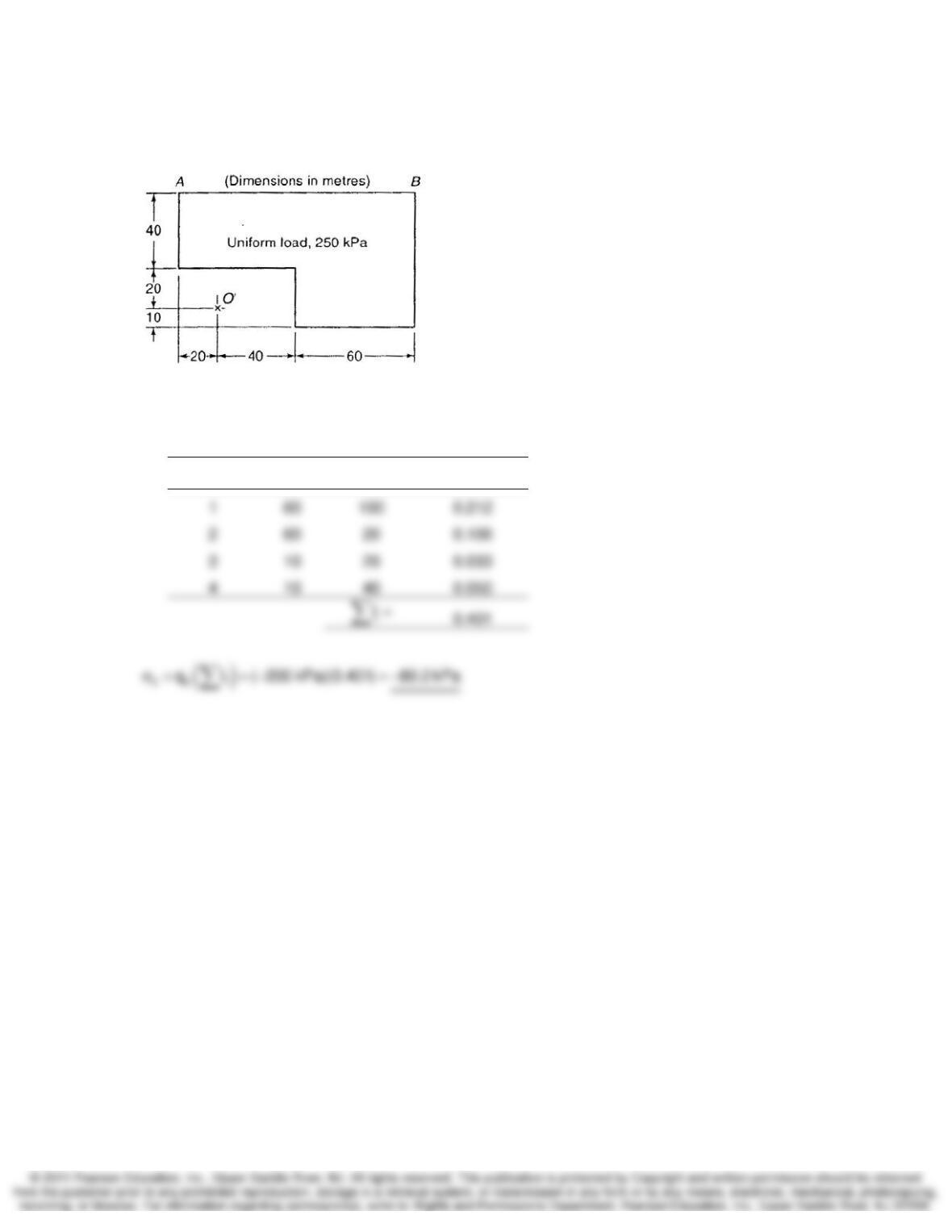
10-10. Given the data of Example 10.6. Instead of a load on the surface, compute the depth of
an excavation to cause a reduction in stress at the bottom of the excavation of 200 kPa if
ρ
= 2.1
Mg/m3. The excavation plan area is shown in Fig. Ex. 10.6a.
SOLUTION:
Find z for Δσ = 200 kPa at point O’ using the Boussinesq method (Fig. 10.4 or Eq. 10.6)
Find σz at z = 9.71 m, for qo = -200 kPa. (Influence values presented in the table below were
determined using the Boussinesq solution as given by Eq. 10.6.)
Rectangle x y I
1 60 100 0.25
Stress Distribution and Settlement Analysis Chapter 10
10-11. For the excavation of Problem 10.10, estimate the stress change at a depth of 50 m
below the bottom of the excavation at point O’.
SOLUTION:
Find σz at z = 50 m, for qo = -200 kPa. (Influence values presented in the table below were
determined using the Boussinesq solution as given by Eq. 10.6.)
Rectangle x y I
qo = -200 kPa, z = 50 m
Determine the stress decrease using
Fig. 10.4 (or Eq. 10.6) for the vertical
stress under the corner of a uniformly
loaded rectangular area. Use
superposition by adding I values for the
4 rectangular areas as tabulated below.
Stress Distribution and Settlement Analysis Chapter 10
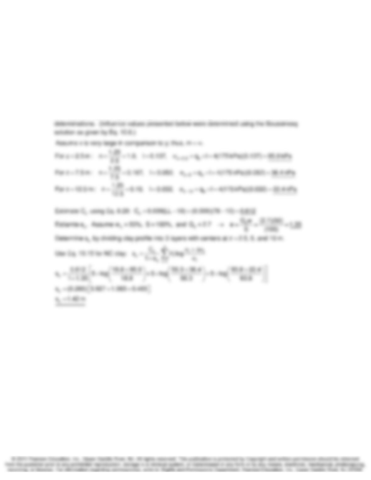
10-13. A strip footing 2.5 m wide is loaded on the ground surface with a pressure equal to 175
kPa. Calculate the stress distribution at depths of 2.5, 7.5 and 12.5 m under the center of the
footing. If the footing rested on a normally consolidated cohesive layer whose LL was 78 and
whose PL was 47, estimate the settlement of the footing. Assume wn = 50%, S = 100%, γ’ = 7.5
kN/m3, and the total clay layer thickness beneath the footing = 15 m.
SOLUTION:
Find σz for qo = 175 kPa. Use ½ the footing width and multiply by 4 (superposition) to determine
the maximum value of σz at the midpoint of the strip footing. Use this value for settlement
Stress Distribution and Settlement Analysis Chapter 10
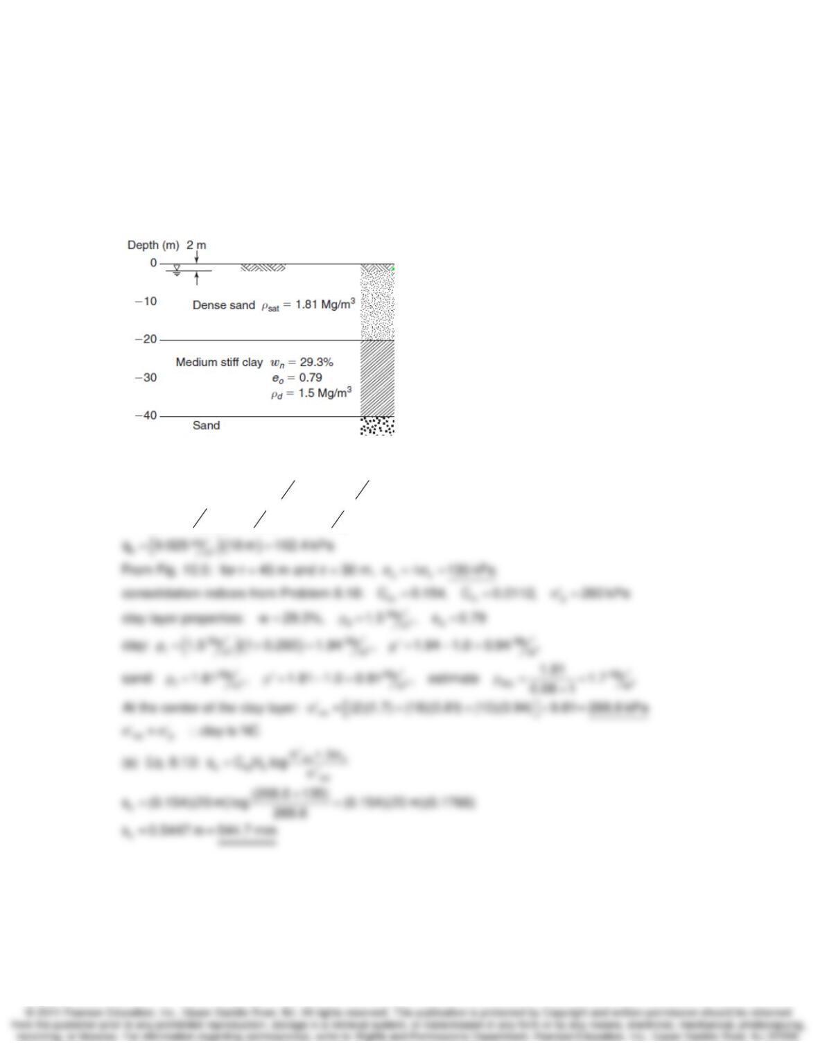
10-16. A large oil storage tank 90 m in diameter is to be constructed on the soil profile shown in
Fig. P10.16. Average depth of the oil in the tank is 18 m, and the specific gravity of the oil is 0.92.
Consolidation tests from the clay layer are similar to those given in Problem 8.18. Estimate the
maximum total and differential consolidation settlement of the tank. Neglect any settlements in
the sand. Work this problem: (a) assuming conditions at the middepth of the clay are typical of
the entire clay layer, and (b) dividing the clay layer into four or five thinner layers, computing the
settlement of each thin layer and summing up by Eq. (8.14). Hint: See Example 10.8.
SOLUTION:
()
()
()
33
32 3
Mg Mg
soil mm
Mg mkN
oil ms m
G 0.92, (0.92) 1 0.92
0.92 9.81 9.025
=ρ= =
γ= =
solution continued on next page
Stress Distribution and Settlement Analysis Chapter 10
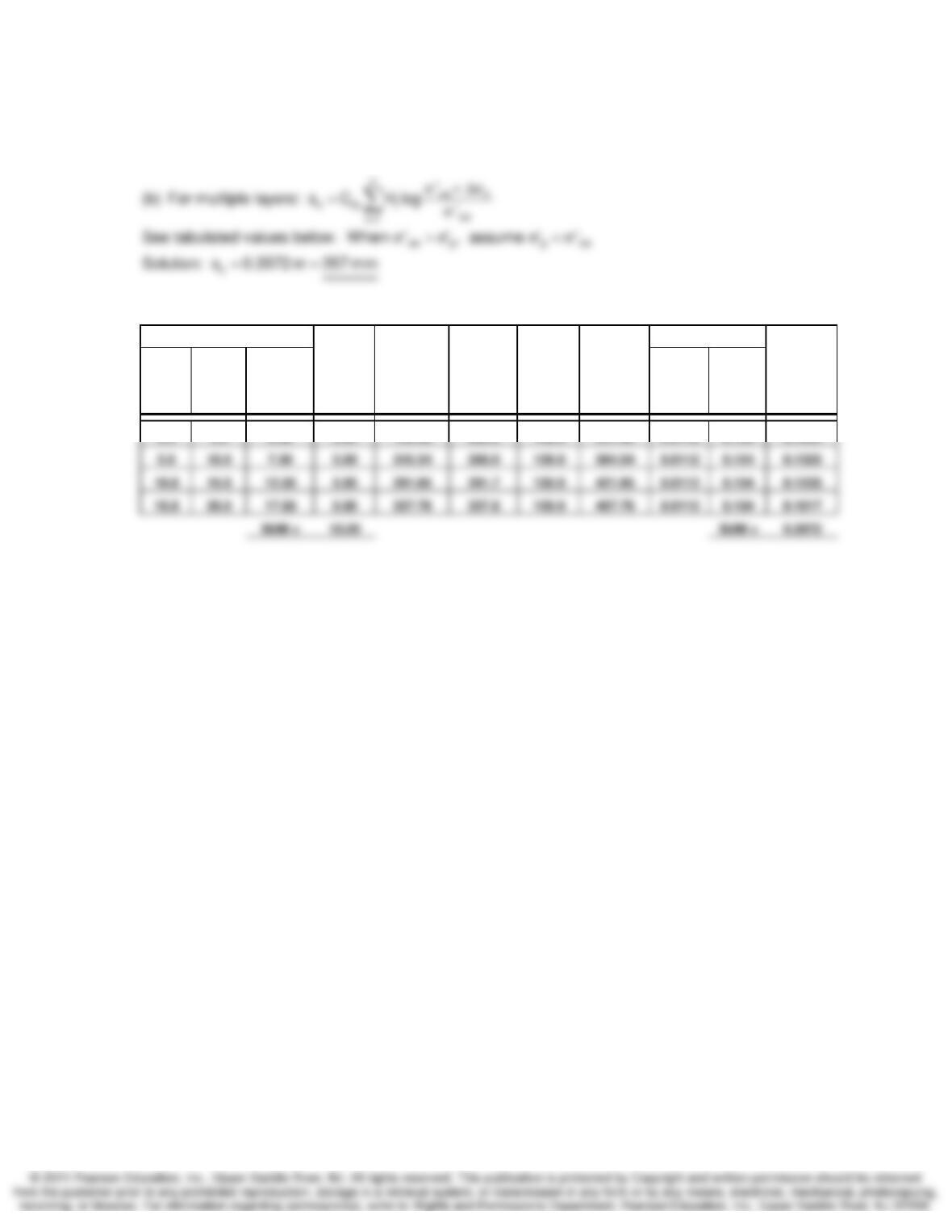
10-16 continued.
Depth Below Clay Surface σ‘
vo
σ‘
p
Δσ
v
σ‘
v
f
Compression Ratio Change in
Sublayer Effective Preconsol. Pressure Final Recomp. Virgin Thickness
Top Bottom Center o
f
Thickness Overburden Pressure Change Pressure Curve Curve
Δ
H
Sublayer H
o
Pressure C
ε
r
C
ε
c
(m) (m) (m) (m) (kPa) (kPa) (kPa) (kPa) (m)
0.0 5.0 2.50 5.00 199.40 260.0 148.0 347.40 0.0112 0.154 0.1034
Stress Distribution and Settlement Analysis Chapter 10
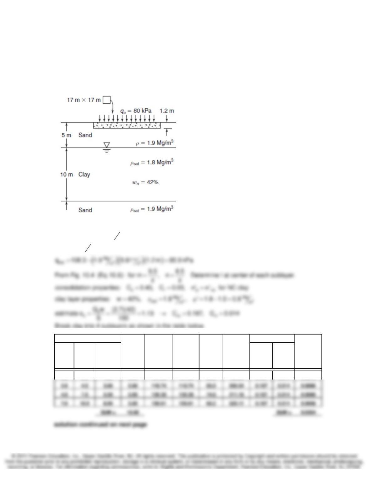
10-17. Estimate the ultimate consolidation settlement under the centerline of a 17 x 17 m mat
foundation. The mat is 1.2 m thick reinforced concrete, and the average stress on the surface of
the slab is 80 kPa. The soil profile is shown in Fig. P10.17. Oedometer tests on samples of the
clay provide these average values: Neglect any settlements due to the sand layer.
C
c = 0.40, Cr = 0.03, clay is NC
SOLUTION:
()
()
3
3
kN
conc m
kN
om
Estimate 23.6
q 23.6 1.2 m 80 108.3 kPa
γ=
=+=
Depth Below Clay Surface σ‘vo σ‘
p
Δσ
v
σ‘vf Compression Ratio Change in
Sublayer Effective Preconsol. Pressure Final Recomp. Virgin Thickness
Top Bottom Center of Thickness Overburden Pressure Change Pressure Curve Curve
Δ
H
Sublayer HoPressure C
ε
rC
ε
c
(m) (m) (m) (m) (kPa) (kPa) (kPa) (kPa) (m)
0.0 2.0 1.00 2.00 101.05 101.05 85.8 186.85 0.187 0.014 0.0075
Stress Distribution and Settlement Analysis Chapter 10
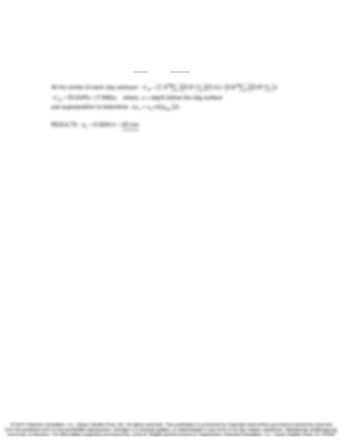
10-17 continued.
n
cii
ci
oi
i1
C
Use Eq. 10.15 for NC clay: s H log
1e
=
σ+Δσ
=+σ
∑