Chapter 1 Homework The Flexural Rigidity The Beam

1

CHAPTER 1

Problem 1.1

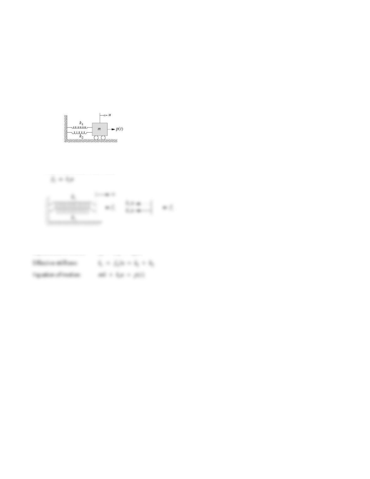
Starting from the basic definition of stiffness, determine

the effective stiffness of the combined spring and write the

equation of motion for the spring–mass systems shown in

Fig. P1.1.

Figure P1.1

Solution:

If

k

e is the effective stiffness,

Equilibrium of forces:

f

k

u

k

f

k

t

f

k

2

Problem 1.2

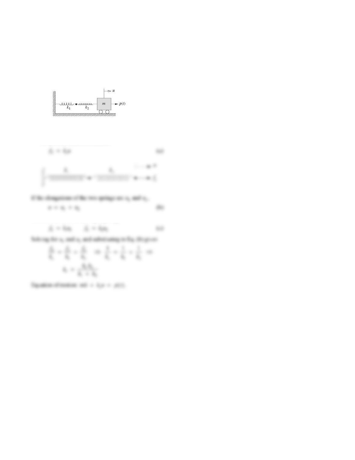
Starting from the basic definition of stiffness, determine

the effective stiffness of the combined spring and write the

equation of motion for the spring–mass systems shown in

Fig. P1.2.

Figure P1.2

Solution:

If

k

e is the effective stiffness,

Because the force in each spring is

f

S,

f

k

f

k

f

k

3

Problem 1.3

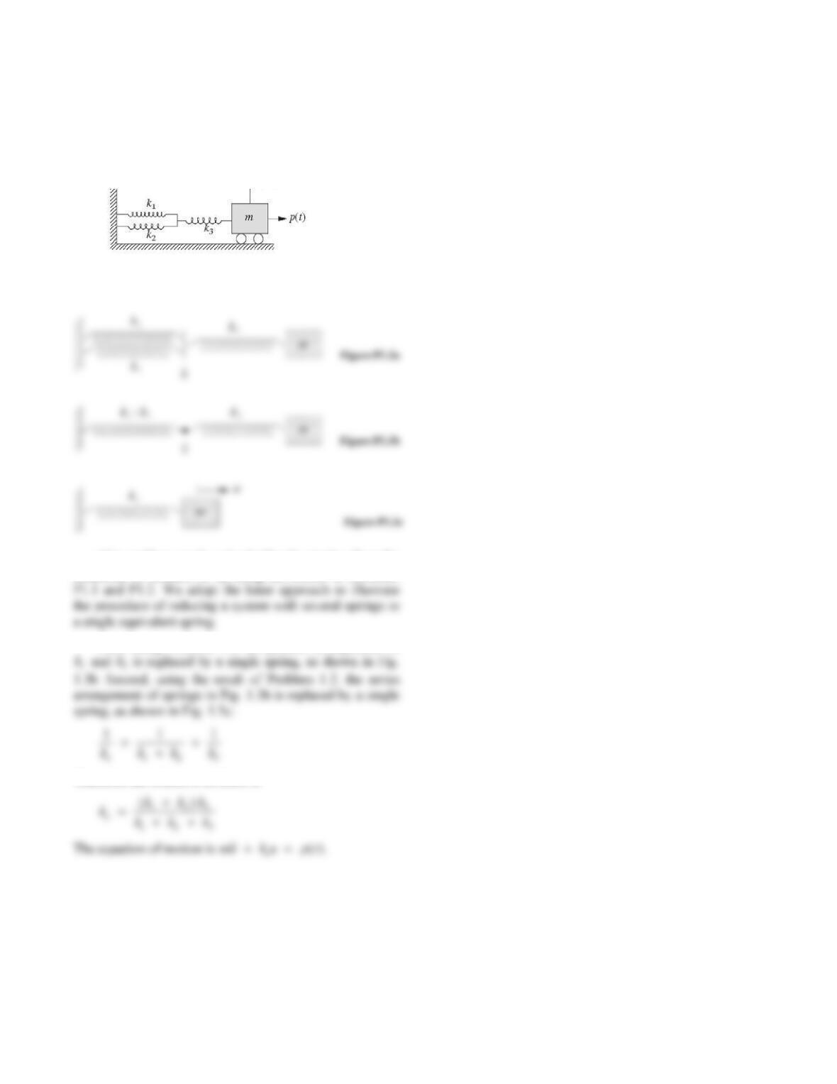
Starting from the basic definition of stiffness, determine

the effective stiffness of the combined spring and write the

equation of motion for the spring–mass systems shown in

Fig. P1.3.

Figure P1.3

Solution:

This problem can be solved either by starting from the

definition of stiffness or by using the results of Problems

First, using Problem 1.1, the parallel arrangement of

Therefore the effective stiffness is

4

Problem 1.4

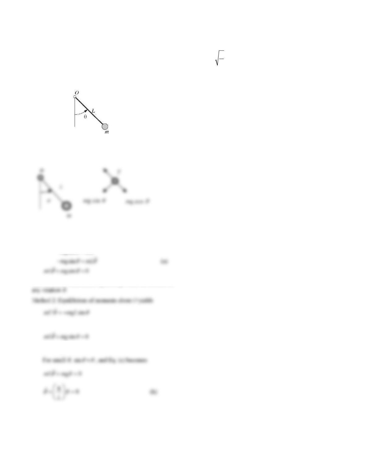
Derive the equation governing the free motion of a simple

pendulum that consists of a rigid massless rod pivoted at

point O with a mass m attached at the tip (Fig. P1.4).

Linearize the equation, for small oscillations, and

determine the natural frequency of oscillation.

Figure P1.4

Solution:

1. Draw a free body diagram of the mass.

2. Write equation of motion in tangential direction.

Method 1: By Newton’s law.

gsin



mma





This nonlinear differential equation governs the motion for

or

3. Linearize for small



.

4. Determine natural frequency.

g

n

L





5

Consider the free motion in the xy plane of a compound

pendulum that consists of a rigid rod suspended from a

point (Fig. P1.5). The length of the rod is L, and its mass m

(b) Linearize the equation for small θ.

Figure P1.5

Solution:

1. Find the moment of inertia about O.

From Appendix 8,

2. Draw a free body diagram of the body in an arbitrary

displaced position.

3. Write the equation of motion using Newton’s second law

4. Specialize for small



.

For small



, sin







and Eq. (a) becomes

5. Determine natural frequency.

6

Problem 1.6

Repeat Problem 1.5 for the system shown in Fig. P1.6,

which differs in only one sense: its width varies from zero

1. Find the moment of inertia about about O.

IrdA

2





2. Draw a free body diagram of the body in an arbitrary

displaced position.

3. Write the equation of motion using Newton’s second law

of motion.

00

MI









4. Specialize for small



.

For small



, sin







, and Eq. (a) becomes

or

5. Determine natural frequency.

k

7

Problem 1.7

Develop the equation governing the longitudinal motion of

the system of Fig. P1.7. The rod is made of an elastic

material with elastic modulus E; its cross-sectional area is

A and its length is L. Ignore the mass of the rod and

measure u from the static equilibrium position.

Figure P1.7

Solution:

Draw a free body diagram of the mass:

Write equation of dynamic equilibrium:

8

Problem 1.8

A rigid disk of mass m is mounted at the end of a flexible

shaft (Fig. P1.8). Neglecting the weight of the shaft and

neglecting damping, derive the equation of free torsional

vibration of the disk. The shear modulus (of rigidity) of the

shaft is G.

Figure P1.8

Solution:

Show forces on the disk:

Write the equation of motion using Newton’s second law

of motion:

Write the torque-twist relation:

9

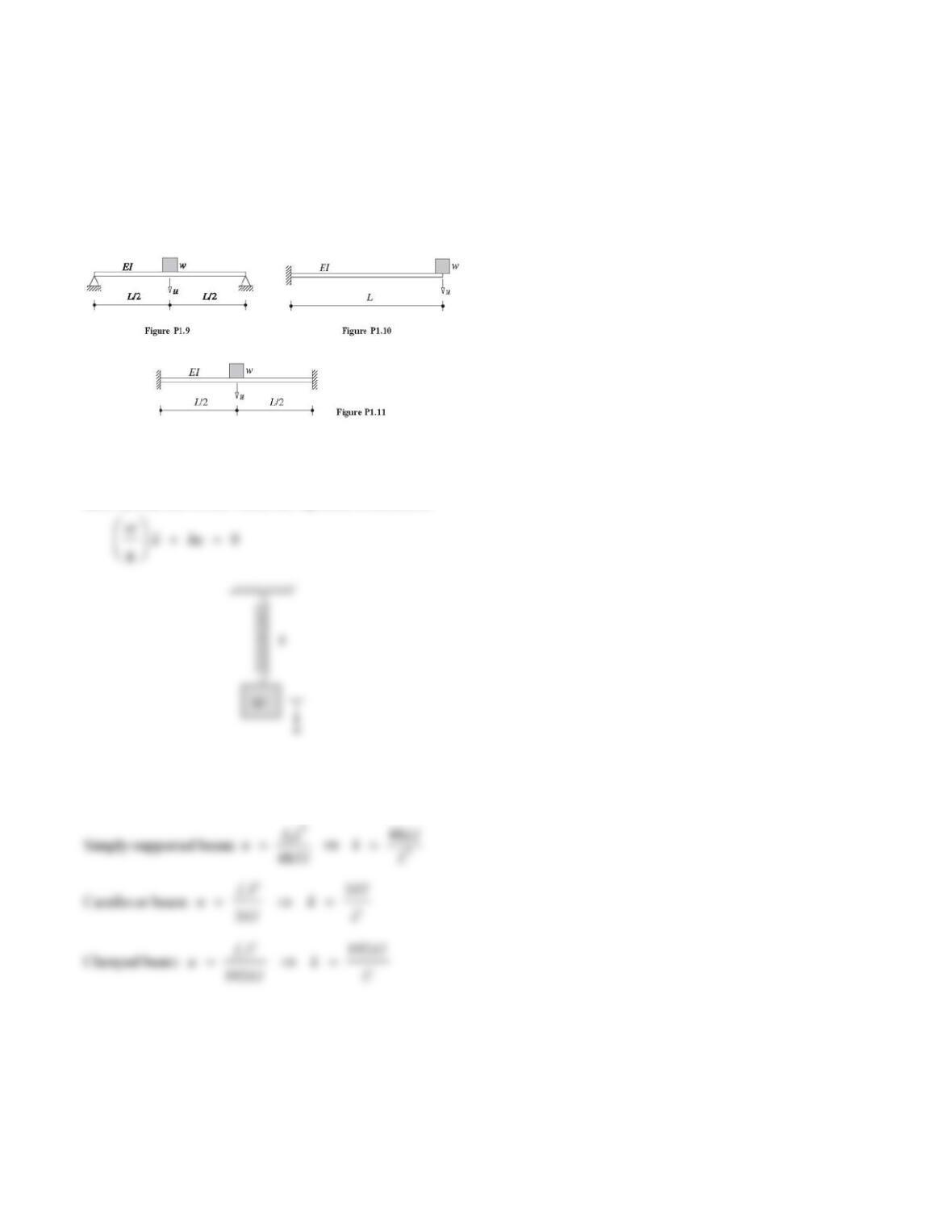
Problems 1.9 through 1.11

Write the equation governing the free vibration of the

systems shown in Figs. P1.9 to P1.11. Assuming the beam

to be massless, each system has a single DOF defined as

the vertical deflection under the weight w. The flexural

rigidity of the beam is EI and the length is L.

Solution:

In each case the system is equivalent to the spring-

mass system shown for which the equation of motion is

The spring stiffness is determined from the deflection u

under a vertical force

f

S applied at the location of the

lumped weight:

10

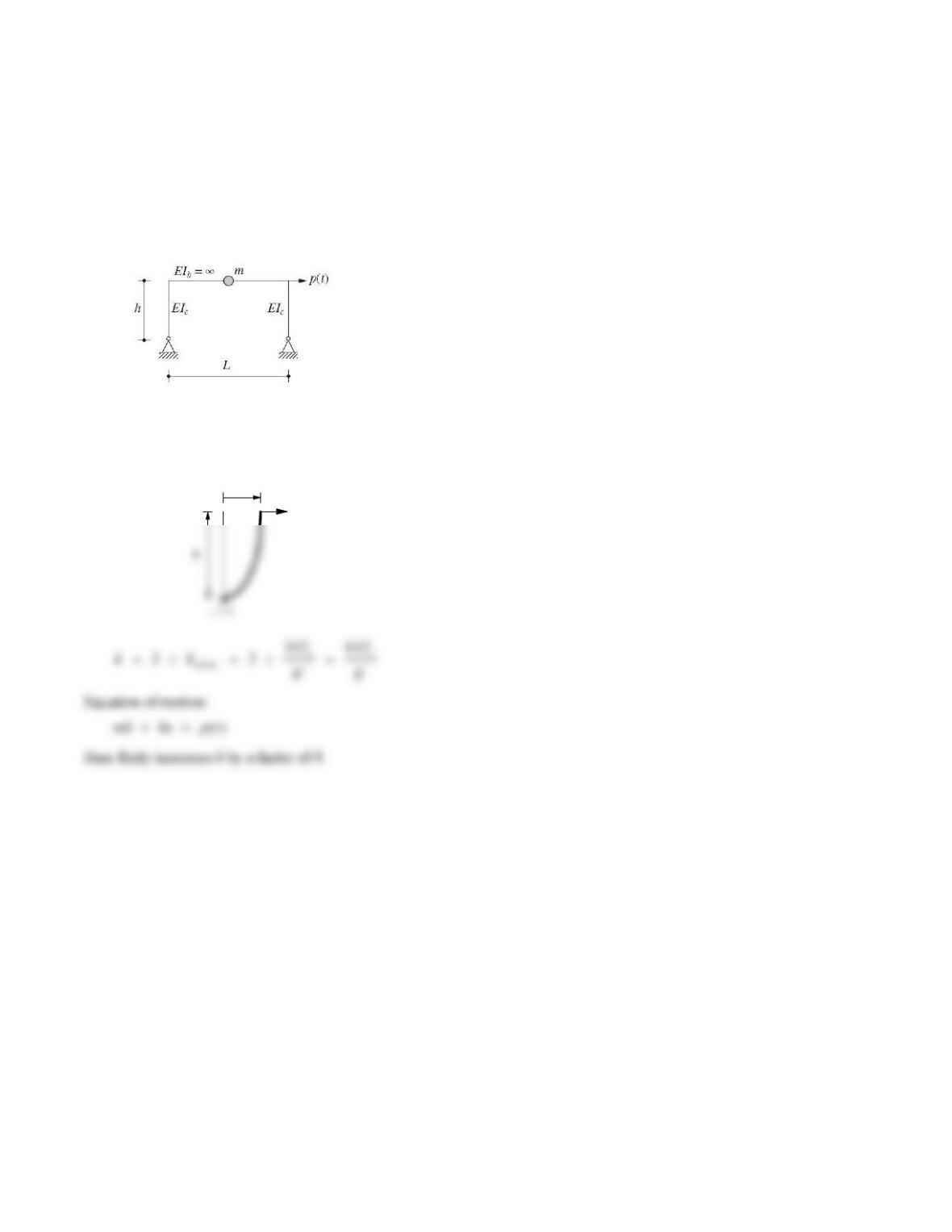
Problem 1.12

(Fig. P1.12). The length of the beam is L, and its flexural

rigidity is EI. The spring stiffness is k. Assume the beam to

Solution:

Figure 1.12b

1. Write the equation of motion.

S

where

2. Determine the effective stiffness.

where

Substitute for the



’s from Eq. (f) and for u from Eq. (d):

3. Determine the natural frequency.

EI

Undeformed position

Simply

w

11

Problem 1.13

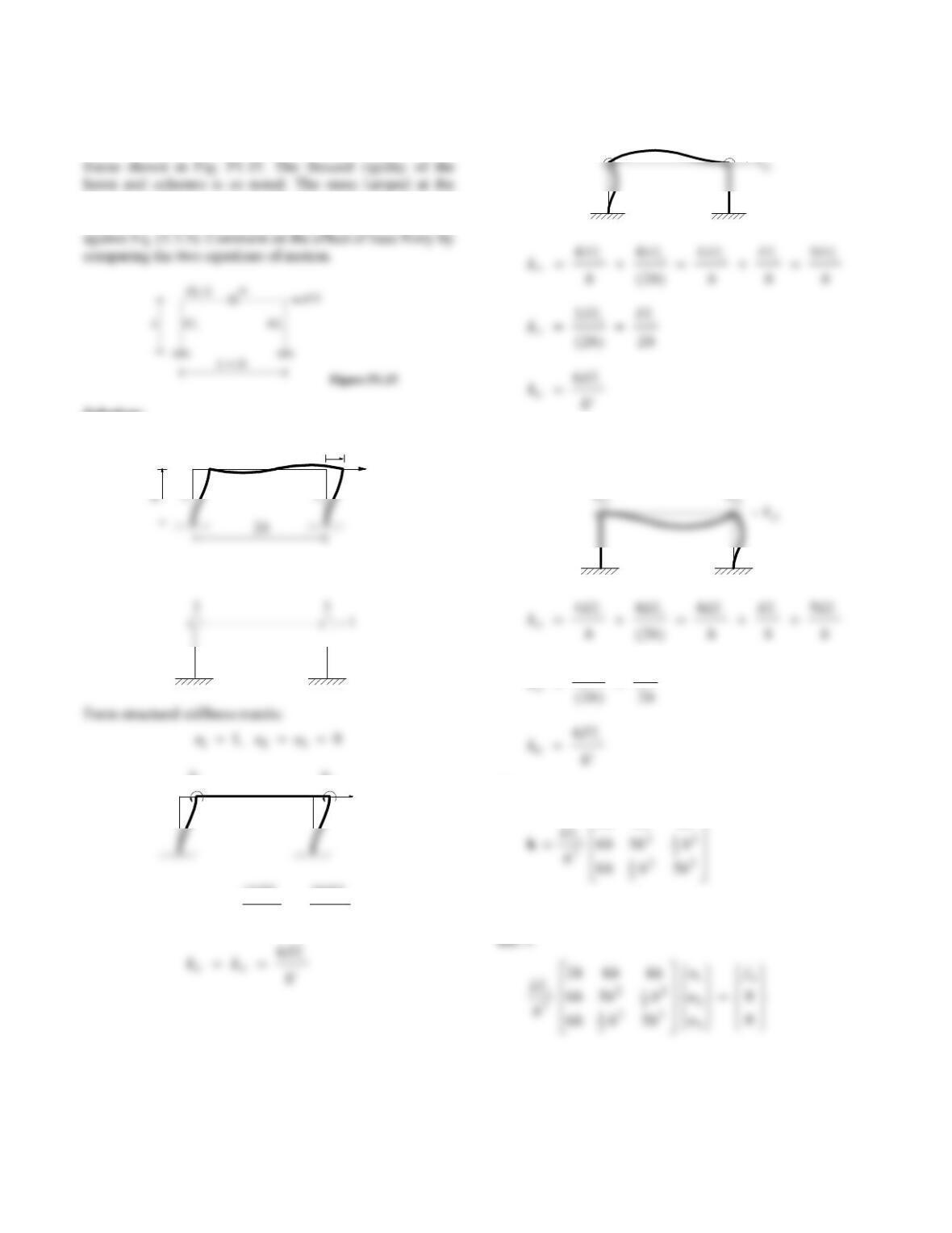
Derive the equation of motion for the frame shown in Fig.

P1.13. The flexural rigidity of the beam and columns is as

noted. The mass lumped at the beam is m; otherwise,

assume the frame to be massless and neglect damping. By

comparing the result with Eq. (1.3.2), comment on the

effect of base fixity.

Figure P1.13

Solution:

Compute lateral stiffness:

1

3EI /h

c

3

Problem 1.14

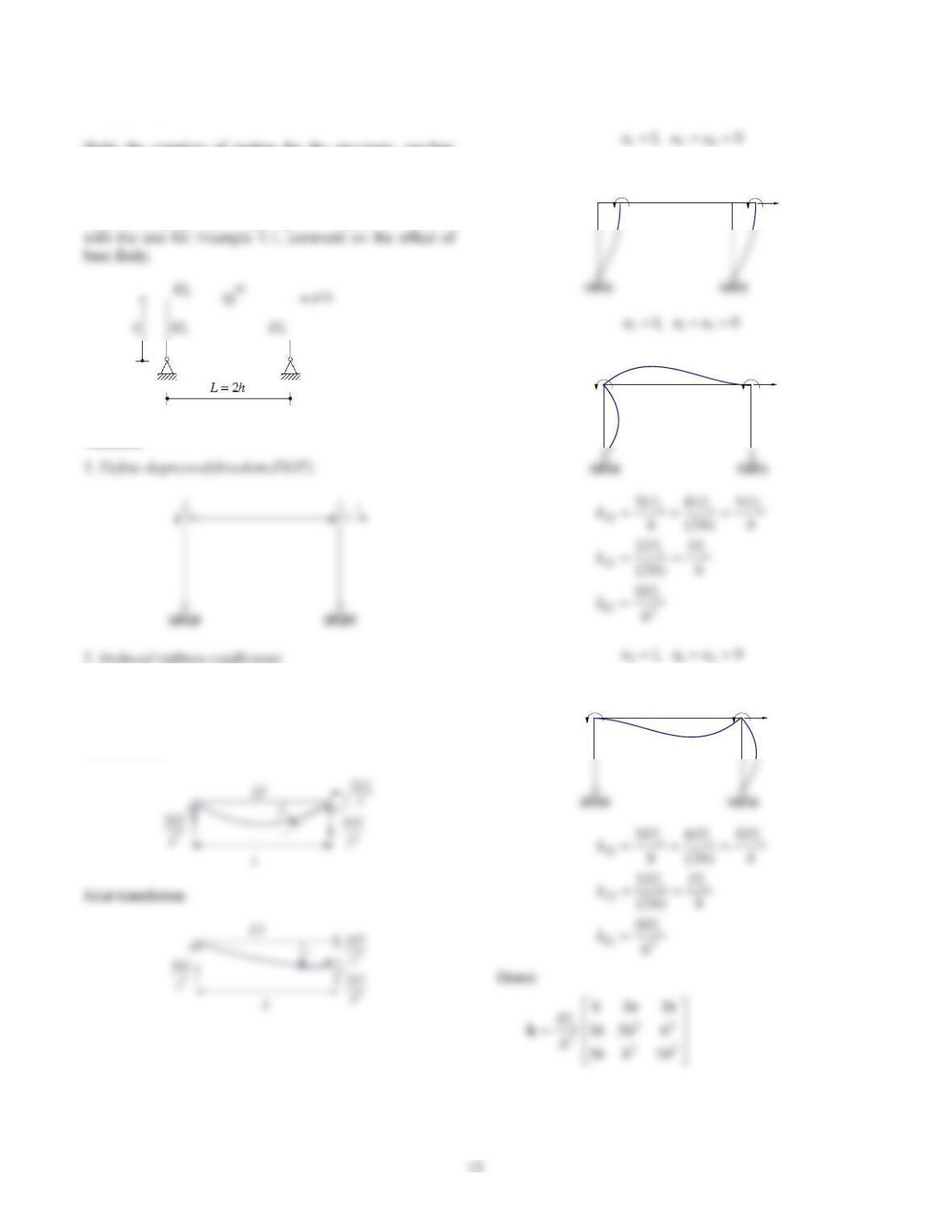
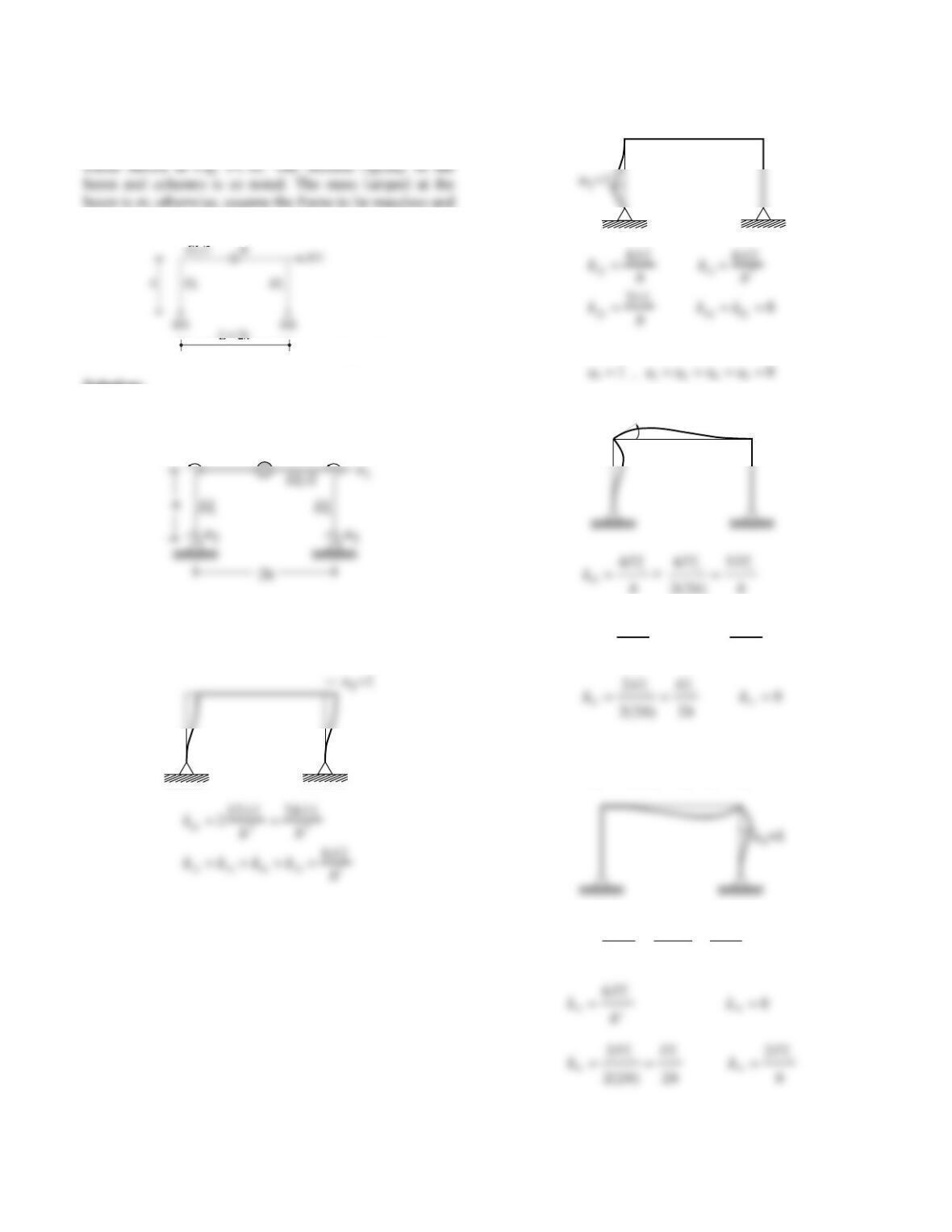
Write the equation of motion for the one-story, one-bay

frame shown in Fig. P1.14. The flexural rigidity of the

beam and columns is as noted. The mass lumped at the

beam is m; otherwise, assume the frame to be massless and

neglect damping. By comparing this equation of motion

Figure P1.14

Solution:

2. Reduced stiffness coefficients.

Since there are no external moments applied at the

pinned supports, the following reduced stiffness

coefficients are used for the columns.

Joint rotation:

3. Form structural stiffness matrix.

123

k21 k31

k22 k23

k13

k23 k33

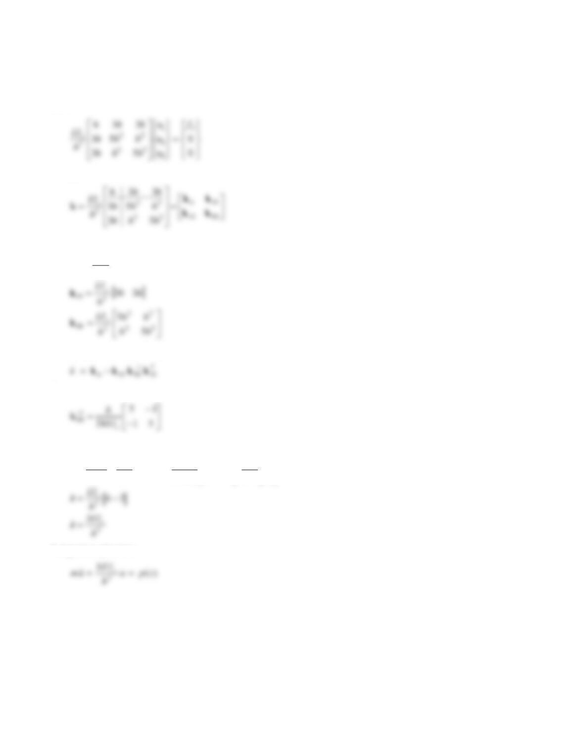
13

4. Determine lateral stiffness.

The lateral stiffness k of the frame can be obtained by

static condensation since there is no force acting on DOF 2

and 3:

First partition k as

where





3

6

h

EI

c

tt

k

Then compute the lateral stiffness k from

Since

we get



kEI

h

EI

hhh h

EI

h

cc

c

  





















63324

51

15

3

33 3

5. Equation of motion.

14

Problem 1.15

Write the equation of motion of the one-story, one-bay

beam is m; otherwise, assume the frame to be massless and

neglect damping. Check your result from Problem 1.15

Solution:

1

k

Ic

I = I /

bc

2

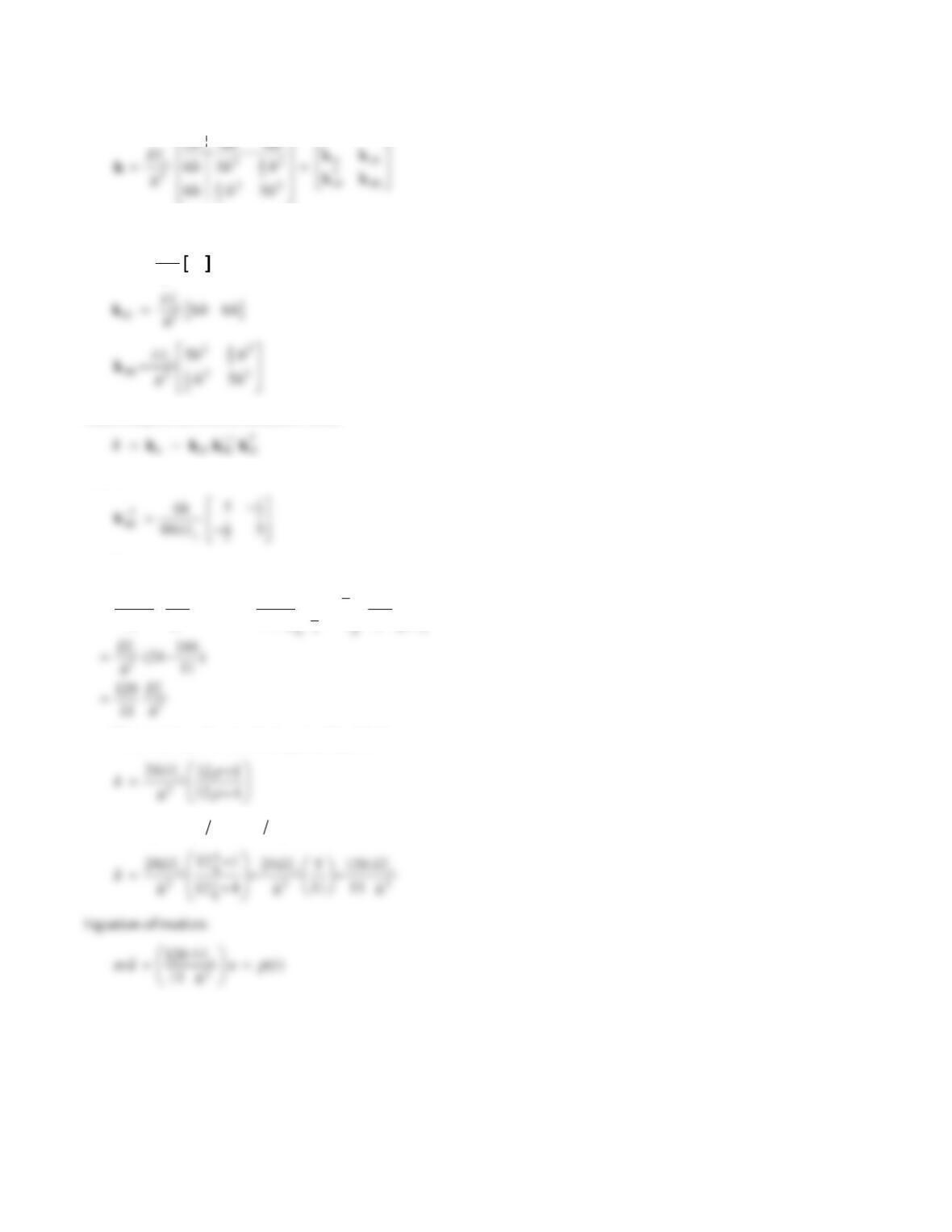
Define degrees-of-freedom (DOF):

k11

k21 k31

11 33

12 24

2

cc

EI EI

k

hh



k

22

k

32

uuu

312

10



,

2

bc

EI EI

Hence





6624

hh

The lateral stiffness k of the frame can be obtained by

static condensation since there is no force acting on DOF 2

uuu

213

10



,

15

First partition k as

where

ktt c

E

I

h

324

I

Then compute the lateral stiffness k from

Since

we get



3

1

2

1

33

6

5

99

4

66

24

h

EI

h

hh

h

EI

h

EI

k

c

cc



























This result can be checked against Eq. 1.3.5:

Substituting





I

bc

418

gives

16

Problem 1.16

Write the equation of motion of the one-story, one-bay

neglect damping.

Figure P1.16

Solution:

1. Define degrees-of-freedom (DOF).

2. Form the structural stiffness matrix.

u11 , u2u3u4u50

u2



1 , u1



u3u4u50



13 23

2

62

cc

EI EI

kk

hh



u4



1 , u1



u2u3u50

44

445

+

2(2 )

ccc

EI EI EI

k

hhh



m

3

u

4

u

3

u =1

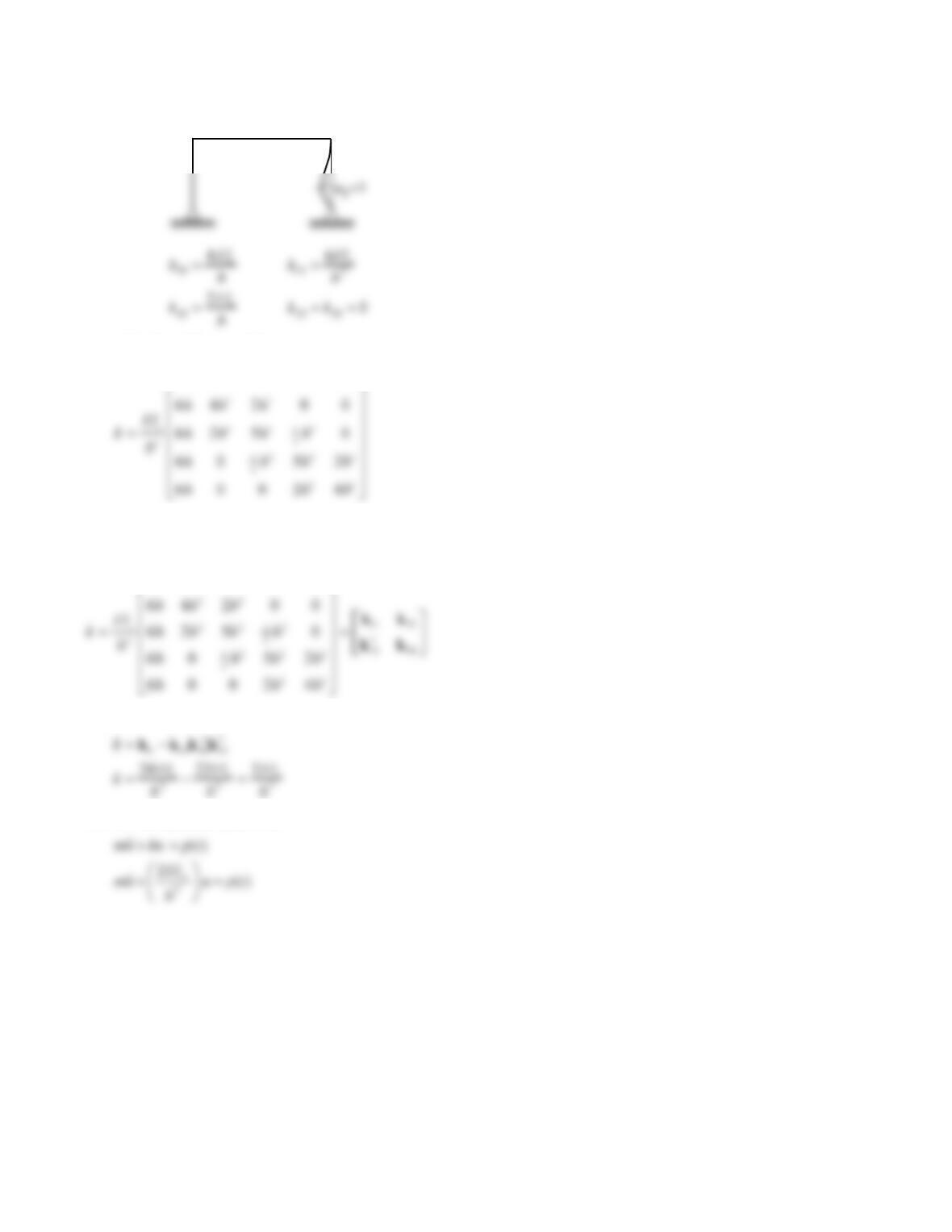
17

u51 , u1u2u3u40

Assemble the stiffness coefficients:

246666

hhhh



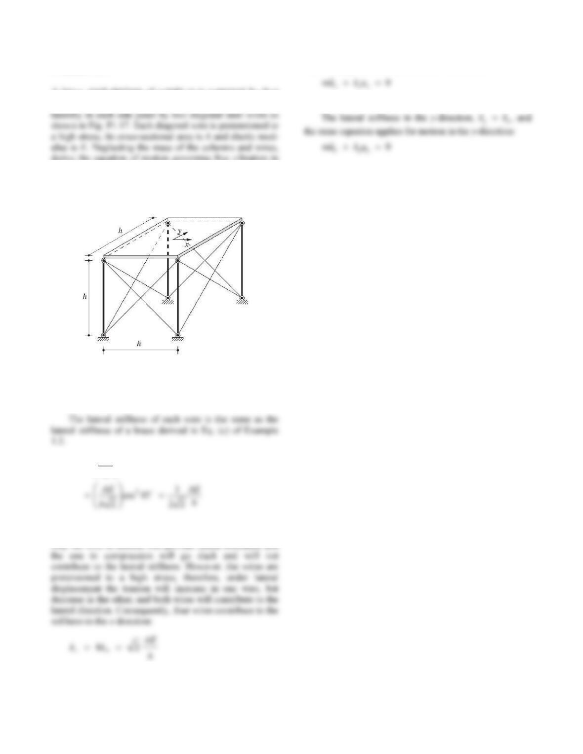
3. Determine the lateral stiffness of the frame.

First partition k.

246666

hhhh



Compute the lateral stiffness.

4. Write the equation of motion.

18

Problem 1.17

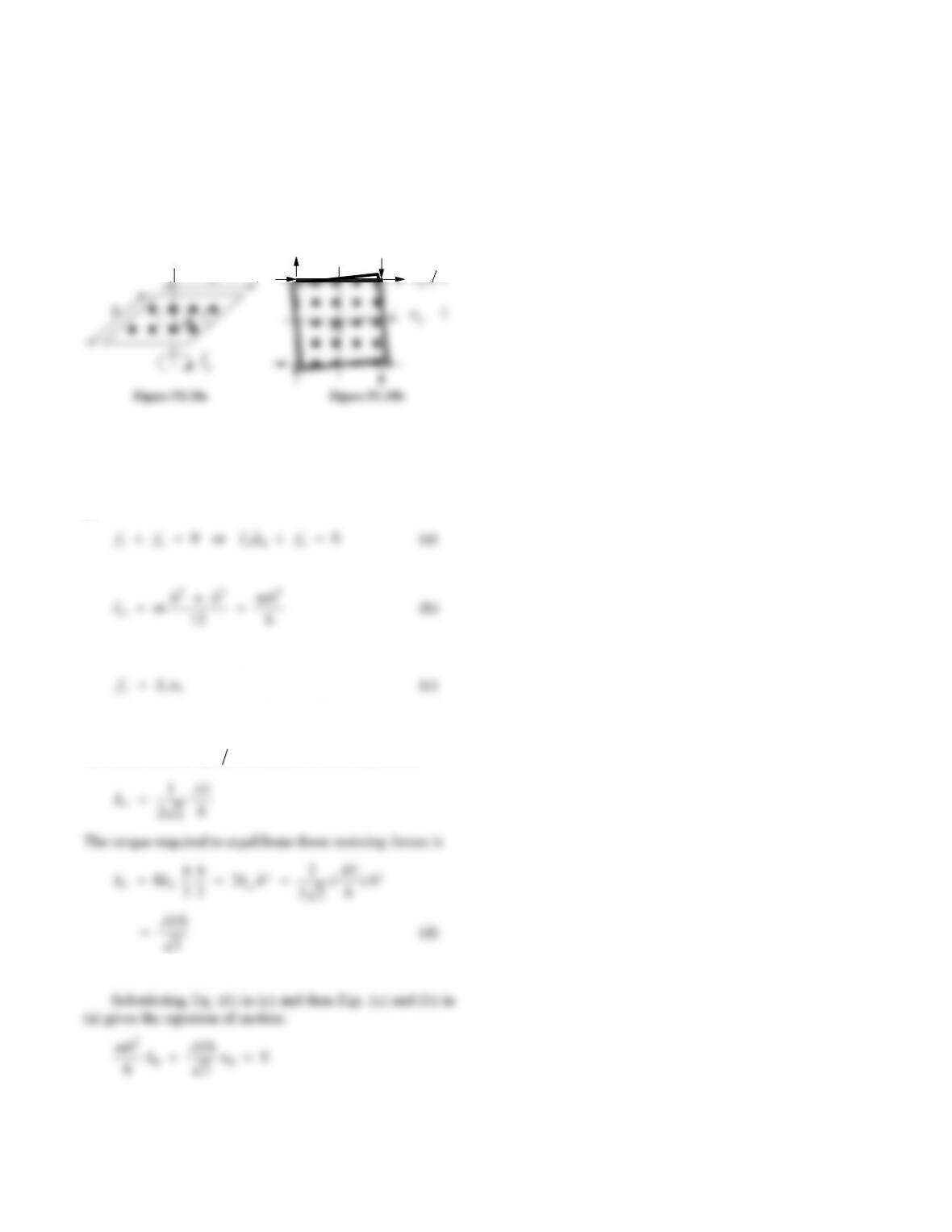
A heavy rigid platform of weight w is supported by four

columns, hinged at the top and the bottom, and braced

derive the equation of motion governing free vibration in

(a) the x-direction, and (b) the y-direction. (Hint: Because

of high pretension, all wires contribute to the structural

stiffness, unlike Example 1.2, where the braces in

compression do not provide stiffness.)

Figure P1.17

Solution:

(a) Equation of motion in the x-direction.

L

AE

kw

cos

2

















Each of the four sides of the structure includes two wires.

If they were not pretensioned, under lateral displacement,

Then the equation of motion in the x-direction is

(b) Equation of motion in the y-direction.

19

Problem 1.18

Derive the equation of motion governing the torsional

vibration of the system of Fig. P1.17 about the vertical axis

passing through the center of the platform.

Solution:

z

h

k h

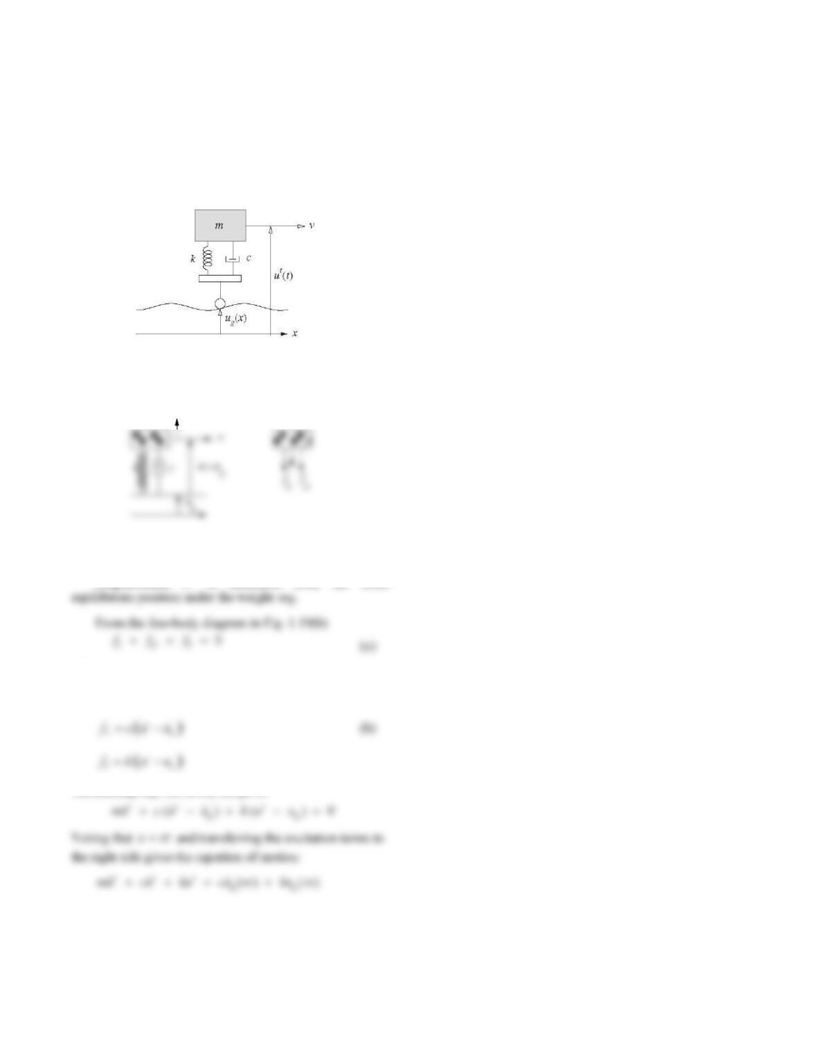
1. Set up equation of motion.

The elastic resisting torque S

f

and inertia force

I

f

are

shown in Fig. 1.18a. The equation of dynamic equilibrium

is

f



where

2. Determine torsional stiffness, k



.

Introduce u



1 in Fig. 1.18b and identify the

resisting forces due to each wire. All the eight forces are

the same; each is 2kh

w, where, from Problem 1.17,

3. Set up equation of motion.

20

Problem 1.19

An automobile is crudely idealized as a lumped mass m

supported on a spring–damper system as shown in Fig.

P1.19. The automobile travels at constant speed v over a

road whose roughness is known as a function of position

along the road. Derive the equation of motion.

Figure P1.19

Solution:

u t

Displacement ut is measured from the static

where

t

I

fmu





Substituting Eqs. (b) in Eq. (a) gives

Figure P1.19a Figure P1.19b