
1
Case #14
“Whirlpool Europe”
Harvard Business School Case #9-202-017 (Rev. November 26, 2002)
Academic instructors who are registered with the publisher’s
website (http://www.hbsp.harvard.edu) may download the Teaching
Note #5-202-124 (Rev. Jan. 14, 2003) for this case free of
charge.
ABSTRACT
Whirlpool Europe manufactures and sells appliances in a
variety of countries in Europe. It considers the investment of
TEACHING OBJECTIVES
The focus of this case is on capital budgeting decision
making involving a technology project which spans several years
and impacts a number of regional markets. As the saying goes,
which are of interest to an engineering manager.
SUGGESTED QUESTIONS FOR CLASSROOM DISCUSSION
1. If an investment in EPR system is made, cash flow is to be
generated by several sources. There are four waves of
implementation specified in the case over the period of 1999 –
2
4. When deciding on the proposed ERP investment, should value be
included for possible cash flow that occurs beyond 2007? What
does it depend on?
5. Would you recommend the ERP investment? What is your major
concern?
ANALYSIS
1. If an investment in EPR system is made, cash flow is to be
generated by several sources. There are four waves of
implementation specified in the case over the period of 1999 –
2007. Calculate the cash flow for all waves due to (a) improved
inventory (one-time, non-taxable), (b) expanded sales due to
better product availability (continuous, taxable), and (c)
enlarged margin (continuous, taxable).
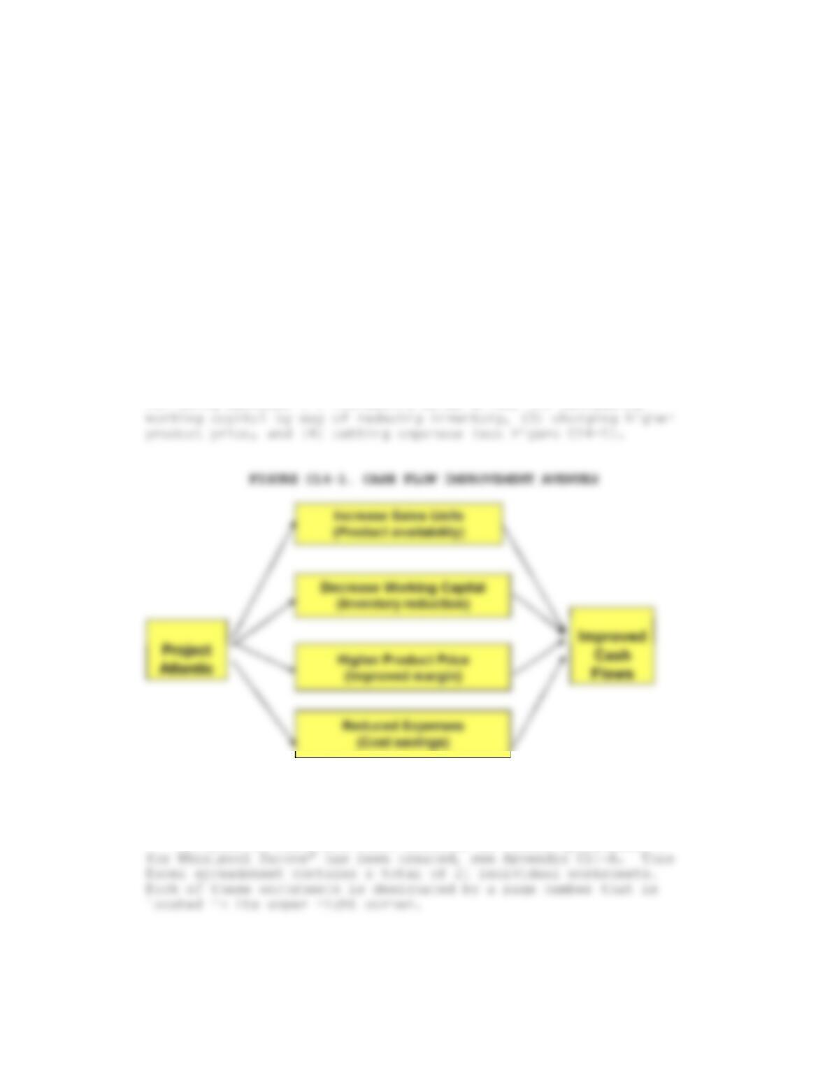
The company’s cash flow may be improved by one or more of the
following methods: (1) increasing sales units, (2) decreasing
The overall approach should be to first determine the added
sales units, the inventory reduction and margin increase for each
region, then to aggregate these inputs in a company-based income
statement to compute the total cash flow.
In order to calculate these results, an “Excel Spreadsheet
The organization of these 21 worksheets is described on page
C14-1. Pages C14-2 and C14-3 summarize important company data
such as capital investments, projected savings in expenses,
projected increases in expenses, Days Sale Inventory (DSI)
upgrades, and margin enhancements.
A. Expanded Sales –Panel D (page C14-5) – For the West region,
pages C14-4 and C14-5 compare the sales units, margin and
inventory levels with and without ERP. Sales are expected to
increase due to increased product availability. Product
availability is to increase from 73.5 percent to 92 percent in
B. Improved Inventory – Panel E (pages C14-5) – Cost of goods
sold (CGS) is equal to the number of products sold in a year
times the unit cost of product. Days Sale Inventory (DSI) is then
defined as:
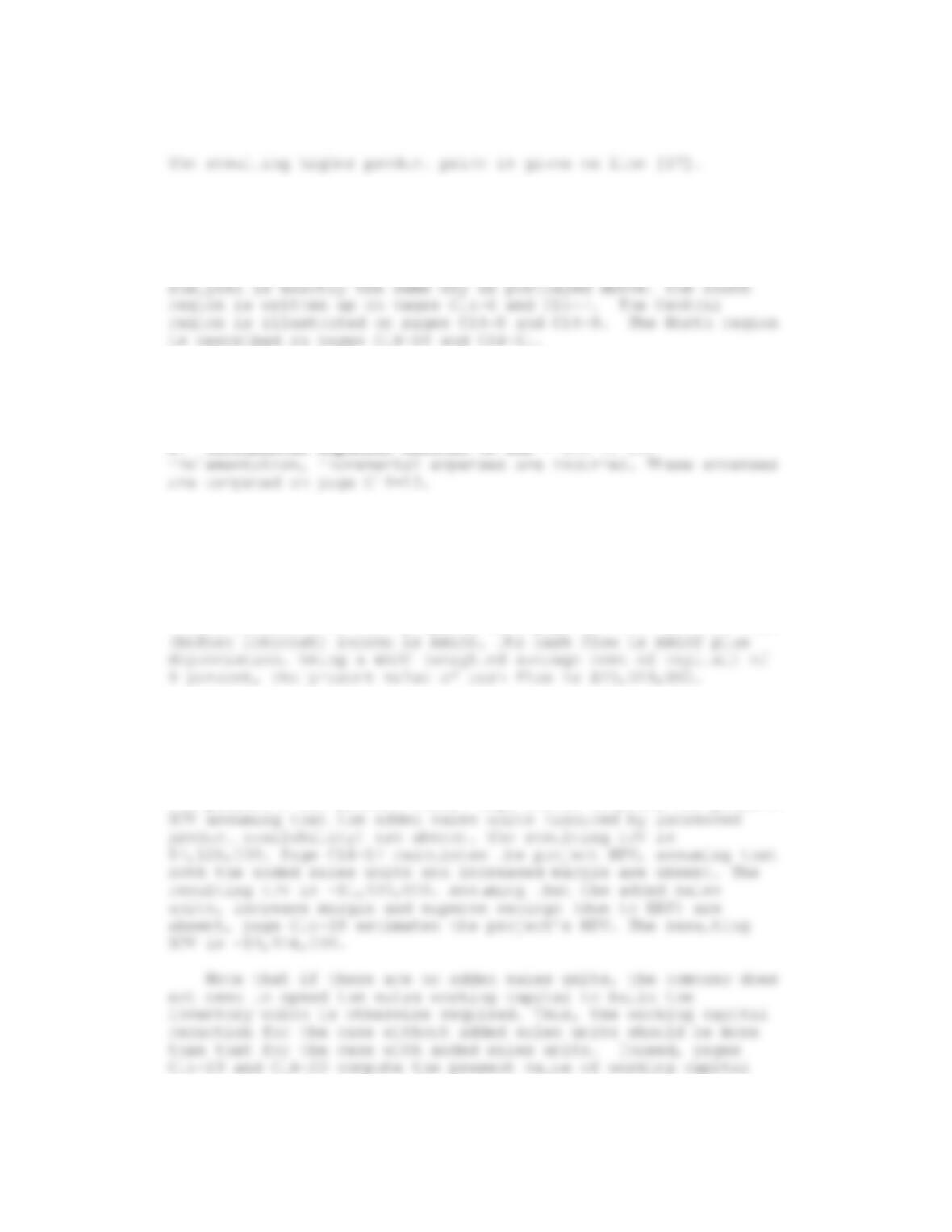
C. Enlarged Margin – Panel C (page C14-4) – For the West region,
the margin increase has been specified for each year on page C14-
2. The improved margin is thus given on line [20] – page C14-4.
4
D. Sales Revenue – The sales revenue with ERP is then computed
by multiplying the new total sales unit (line [13]) with the new
product price (line [17]), as given on line [14].
E. Other Regions – The three other regions are to be modeled and
F. Working Capital Reduction – Because the inventory is scaled
down, less working capital is needed to build inventory. This
working capital reduction is calculated on page C14-12.
G. Incremental Expenses Related to ERP – Due to ERP
H. Depreciation – Depreciation charges must be calculated in
accordance with the activation schedule of the capital investment
involved. The annual deprecation charges are calculated on page
C16-14.
I. Income Statement – Using the above inputs, the company’s
income statement is then prepared (see page C1415). The after-tax
2. Analyze the interactions between these three sources of cash
flow. What is your finding?
The best way to study the interactions between these three
sources of cash flow is to determine their individual impacts on
the project’s net present value. Page C14-16 computes the project
Page C14-21 compares the above individual cases and the
results are summarized in Table C14-1.
TABLE C14-1. SUMMARY OF RESULTS
Cases Total
Capital
Cash Flow
from
Working
Capital
NPV
Investment Operation Reduction
due
and Expenses to
Inventory
1. NPV (all
inclusive) – Page
C14-15
($22,036) $23,319 $22,596 $23,879
By analyzing the results, it becomes clear that: (1) expense
savings contributes $8,639,000; (2) margin enhancement is worth
$8,461,000; (3) added sales units are valued at $16,753,000 of
which $18,726,000 was created by cash flow alone, with $1,973,000
to compensate for working capital reduction; (4) the residual
“basic gain” amounts to be $11,817,000. This is contributed by
the synergy of/from the ERP project.
3. Calculate the present value of the combined after-tax cash
flow from these three sources for the period of 1999 – 2007.
As presented on page C14-15, the working capital reduction is
4. When deciding on the proposed ERP investment, should value be
included for possible cash flow that occurs beyond 2007? What
does it depend on?
6
Value should not be included in this case for several
reasons: (1) the NPV calculated is a positive number large enough
to justify the Project Atlantic; there is no need to include
relatively small due to discounting.
5. Would you recommend the ERP investment? What is your major
concern?
The decision should be in favor of going forward with the ERP
project as its NPV is strongly positive. There are, however,
several major concerns.
A. The sales unit addition is based on the assumption that 25
C. How certain are they that the ERP system be able to deliver
7
APPENDIX C14-A.EXCEL SPREADSHEET FOR WHIRLPOOL EUROPE
Whirlpool Europe Case – HBS #9-202-017 (Rev. November 2002)
Page C14-1
(Dr. C. M. Chang)
Organization of
Worksheets
Pages Contents
C14-1 Organization of Worksheets
C14-2 and C14-3 Company Data
C14-12 Working Capital Reduction
C14-13 Incremental Operating Expenses
C14-14 Depreciation Charges
8
Whirlpool Europe
Case – Company
Data
Page
C14-2
(Dr. C. M.
Chang)
Cost of
Capital 9%
Corporate
Tax 40%
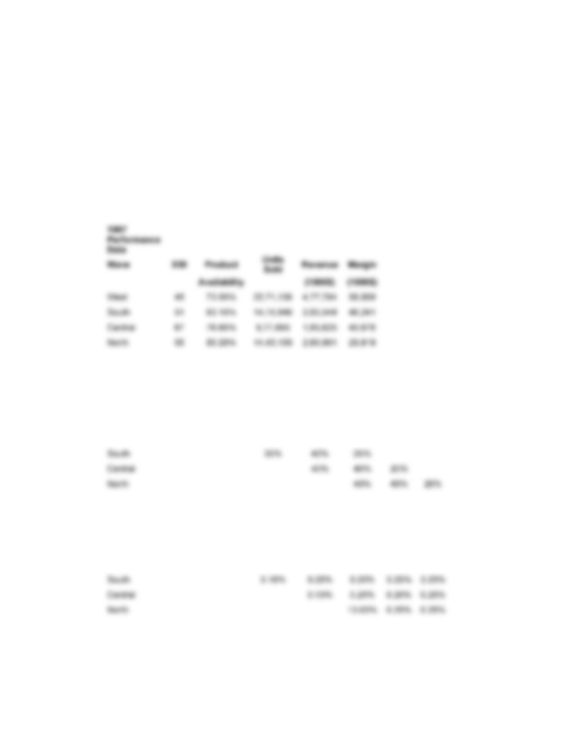
Improvement in DSI and Product Availability
by Year by Wave
1999 2000 2001 2002 2003 2004 2005
West 25% 40% 35%
Cumulative Margin Improvement
by Year by Wave
1999 2000 2001 2002 2003 2004 2005
West 0.06% 0.25% 0.25% 0.25% 0.25% 0.25%
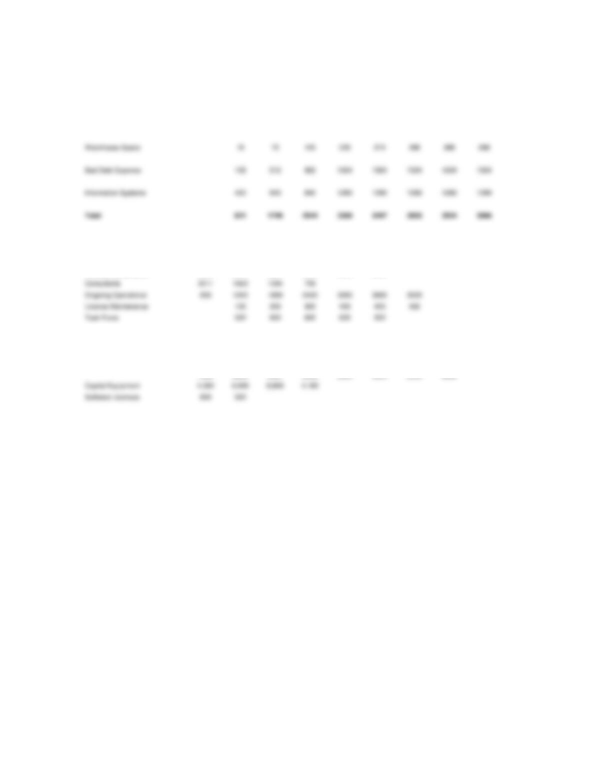
1999 2000 2001 2002 2003 2004 2005 2006 2007
Order Desk Headcount 0 190 411 442 474 506 537 569
Finance Headcount 81 135 216 324 405 405 405 405
Increased Expenses (1000$)
1999 2000 2001 2002 2003 2004 2005 2006 2007
Whirlpool Employees 2250 2250 2250 2250 2250 2250
Ongoing Operational 600 1200 1800 2400 3000 3000 3000
License Maintenance 100 200 300 400 400 400
Task Force 300 600 600 600 300
Total Increased Expenses 6361.2 5513.2 6143.6 6289.2 6250 5950 3400
Investment
1999 2000 2001 2002 2003 2004 2005 2006
Capital Equipment 4,300 8,600 6,900 4,100
Software Licenses 600 300
Total Capital Expenditures 4,900 8,900 6,900 4,100 0 0 0
Projected Other Expense Savings by Year (1000$)
Page C14-3
Warehouse Space 18 72 155 230 274 288 288 288
Bad Debt Expense 102 512 922 1024 1024 1024 1024 1024
Information Systems 420 840 840 1280 1280 1280 1280 1280
1. West Wave
Source/Formula 2000 2001 2002 2003 2004 2005
Panel A: Base Case (Without ERP)
Units [1] = Exhibit 3 2271 2271 2271 2271 2271 2271
Revenue [2] = Exhibit 3 $477,784 $477,784 $477,784 $477,784 $477,784 $477,784
Panel B: Impact of ERP
Additional Units [11] = [29] 36 57 50 0 0 0
Additional Margin [12] = Exhibit 3 0.06% 0.25% 0.25% 0.25% 0.25% 0.25%
DSI Reduction [12A] = [33] 3 8 12 12 12 12
Panel C: Forecast with ERP
Units [13] = [1] + [11] 2307 2364 2414 2414 2414 2414
Revenue [14] = [13] * [17] $485,698 $498,779 $509,329 $509,329 $509,329 $509,329
Cost of Goods Sold (CGS) [15] = [13] * [18] $425,572 $436,087 $445,311 $445,311 $445,311 $445,311
Margin [16] = [13] * [19] $60,125 $62,692 $64,018 $64,018 $64,018 $64,018
Price/unit [17] = [6]*(1 – [20]) $210.53 $210.99 $210.99 $210.99 $210.99 $210.99
CGS/unit [18] = [6] $184.47 $184.47 $184.47 $184.47 $184.47 $184.47
Margin/Unit [19] = [17] – [18] $26.06 $26.52 $26.52 $26.52 $26.52 $26.52
Margin Percentage [20] = [8] + [12] 0.1238 0.1257 0.1257 0.1257 0.1257 0.1257
Days Sales Inventory (DSI) [21] = [9] – [12A] 42 37 33 33 33 33
Inventory [22] = [21]* [15]/365 $48,970 $44,206 $40,261 $40,261 $40,261 $40,261
Whirlpool Europe Case (Dr. C. M. Chang)
Page14-4
Cost of Goods Sold (CGS) [3] = [2] – [4] $418,925 $418,925 $418,925 $418,925 $418,925 $418,925
Margin [4]= Exhibit 3 $58,859 $58,859 $58,859 $58,859 $58,859 $58,859
Price/unit [5] = [2]/[1] $210.38 $210.38 $210.38 $210.38 $210.38 $210.38
CGS/unit [6] = [3]/[1] $184.47 $184.47 $184.47 $184.47 $184.47 $184.47
Margin/Unit [7] = [4]/[1] $25.92 $25.92 $25.92 $25.92 $25.92 $25.92
Margin Percentage [8] = [7]/[5] 12.32% 12.32% 12.32% 12.32% 12.32% 12.32%
Days Sales Inventory (DSI) [9] = Exhibit 3 45 45 45 45 45 45
Inventory [10] = [3]*[9]/365 $51,648 $51,648 $51,648 $51,648 $51,648 $51,648
Panel D: Calculation of Additional Units
Page C14-5
Units
Pre-ERP units [23] = [1] 2271 2271 2271 2271 2271 2271
Pre-ERP Availability [24] = Exhibit 3 0.735 0.735 0.735 0.735 0.735 0.735
Target Availability [25] = Case data 0.92 0.92 0.92 0.92 0.92 0.92
Increase in Availability [26] = ([25]-[24])/[24] 25.17% 25.17% 25.17% 25.17% 25.17% 25.17%
Additional Sales [27]= Case 25.00% 25.00% 25.00% 25.00% 25.00% 25.00%
Percentage Improvement [28] = Exhibit 4 25% 40% 35% 0% 0% 0%
Additional Units [29] = [23}*[26]* 36 57 50 0 0 0
Savings
Target DSI Reduction [30] = Case data 12 12 12 12 12 12
Percentage Improvement [31] = Exhibit 4 25% 40% 35% 0% 0% 0%
DSI Reduction in Year [32] = [30] * [31] 3 4.8 4.2 0 0 0
DSI Reduction [33] = Cumulative [32] 3 8 12 12 12 12

2. South Wave
Source/Formula 2000 2001 2002 2003 2004 2005
Panel A: Base Case (Without ERP)
Units [1] = Exhibit 3 1416 1416 1416 1416 1416 1416
Revenue [2] = Exhibit 3 $283,549 $283,549 $283,549 $283,549 $283,549 $283,549
Cost of Goods Sold (CGS) [3] = [2] – [4] $237,308 $237,308 $237,308 $237,308 $237,308 $237,308
Panel B: Impact of ERP
Additional Units [11] = [29] 0 13 15 9 0 0
Additional Margin [12] = Exhibit 3 0.00% 0.10% 0.25% 0.25% 0.25% 0.25%
DSI Reduction [12A] = [33] 0 4 9 12 12 12
Panel C: Forecast with ERP
Units [13] = [1] + [11] 1416 1429 1444 1454 1454 1454
Revenue [14] = [13] * [17] $283,548 $286,494 $290,022 $292,030 $292,030 $292,030
Cost of Goods Sold (CGS) [15] = [13] * [18] $237,307 $239,486 $242,000 $243,676 $243,676 $243,676
Margin [16] = [13] * [19] $46,241 $47,008 $48,022 $48,354 $48,354 $48,354
Price/unit [17] = [6]*(1 – [20]) $200.25 $200.49 $200.85 $200.85 $200.85 $200.85
CGS/unit [18] = [6] $167.59 $167.59 $167.59 $167.59 $167.59 $167.59
Margin/Unit [19] = [17] – [18] $32.66 $32.90 $33.26 $33.26 $33.26 $33.26
Margin Percentage [20] = [8] + [12] 0.1631 0.1641 0.1656 0.1656 0.1656 0.1656
Days Sales Inventory (DSI) [21] = [9] – [12A] 51 47 42 39 39 39
Inventory [22] = [21]* [15]/365 $33,158 $30,838 $27,847 $26,037 $26,037 $26,037
Whirlpool Europe Case (Dr. C. M. Chang)
Page C14-6
Margin [4]= Exhibit 3 $46,241 $46,241 $46,241 $46,241 $46,241 $46,241
Price/unit [5] = [2]/[1] $200.25 $200.25 $200.25 $200.25 $200.25 $200.25
CGS/unit [6] = [3]/[1] $167.59 $167.59 $167.59 $167.59 $167.59 $167.59
Margin/Unit [7] = [4]/[1] $32.66 $32.66 $32.66 $32.66 $32.66 $32.66
Margin Percentage [8] = [7]/[5] 16.31% 16.31% 16.31% 16.31% 16.31% 16.31%
Days Sales Inventory (DSI) [9] = Exhibit 3 51 51 51 51 51 51
Inventory [10] = [3]*[9]/365 $33,158 $33,158 $33,158 $33,158 $33,158 $33,158
Panel D: Calculation of Additional Units
PageC14- 7
Units
Pre-ERP units [23] = [1] 1416 1416 1416 1416 1416 1416
Pre-ERP Availability [24] = Exhibit 3 0.831 0.831 0.831 0.831 0.831 0.831
Target Availability [25] = Case data 0.92 0.92 0.92 0.92 0.92 0.92
Increase in Availability [26] = ([25]-[24])/[24] 10.71% 10.71% 10.71% 10.71% 10.71% 10.71%
Additional Sales [27]= Case 25.00% 25.00% 25.00% 25.00% 25.00% 25.00%
Percentage Improvement [28] = Exhibit 4 0% 35% 40% 25% 0% 0%
Additional Units [29] = [23}*[26]* 0 13 15 9 0 0
Target DSI Reduction [30] = Case data 12 12 12 12 12 12
Percentage Improvement [31] = Exhibit 4 0% 35% 40% 25% 0% 0%
3. Central Wave
Source/Formula 2000 2001 2002 2003 2004 2005
Units [1] = Exhibit 3 978 978 978 978 978 978
Revenue [2] = Exhibit 3 $185,625 $185,625 $185,625 $185,625 $185,625 $185,625
Cost of Goods Sold (CGS) [3] = [2] – [4] $141,947 $141,947 $141,947 $141,947 $141,947 $141,947
Margin [4]= Exhibit 3 $43,678 $43,678 $43,678 $43,678 $43,678 $43,678
Panel C: Forecast with ERP
Units [13] = [1] + [11] 978 978 997 1016 1026 1026
Revenue [14] = [13] * [17] $185,702 $185,702 $189,632 $193,550 $195,455 $195,455
Cost of Goods Sold (CGS) [15] = [13] * [18] $142,006 $142,006 $144,764 $147,523 $148,975 $148,975
Margin [16] = [13] * [19] $43,696 $43,696 $44,867 $46,027 $46,480 $46,480
Price/unit [17] = [6]*(1 – [20]) $189.88 $189.88 $190.20 $190.50 $190.50 $190.50
CGS/unit [18] = [6] $145.20 $145.20 $145.20 $145.20 $145.20 $145.20
Margin/Unit [19] = [17] – [18] $44.68 $44.68 $45.00 $45.30 $45.30 $45.30
Margin Percentage [20] = [8] + [12] 0.2353 0.2353 0.2366 0.2378 0.2378 0.2378
Days Sales Inventory (DSI) [21] = [9] – [12A] 67 67 62.2 57.4 55 55
Inventory [22] = [21]* [15]/365 $26,067 $26,067 $24,669 $23,200 $22,448 $22,448
Whirlpool Europe Case (Dr. C. M. Chang)
Page C14- 8
Panel A: Base Case (Without ERP)
Price/unit [5] = [2]/[1] $189.80 $189.80 $189.80 $189.80 $189.80 $189.80
CGS/unit [6] = [3]/[1] $145.14 $145.14 $145.14 $145.14 $145.14 $145.14
Margin/Unit [7] = [4]/[1] $44.66 $44.66 $44.66 $44.66 $44.66 $44.66
Margin Percentage [8] = [7]/[5] 23.53% 23.53% 23.53% 23.53% 23.53% 23.53%
Days Sales Inventory (DSI) [9] = Exhibit 3 67 67 67 67 67 67
Inventory [10] = [3]*[9]/365 $26,056 $26,056 $26,056 $26,056 $26,056 $26,056
Panel B: Impact of ERP
Additional Margin [12] = Exhibit 3 0.00% 0.00% 0.13% 0.25% 0.25% 0.25%
DSI Reduction [12A] = [33] 0 0 4.8 9.6 12 12