142
Chapter 10
Capital Markets and the Pricing of Risk
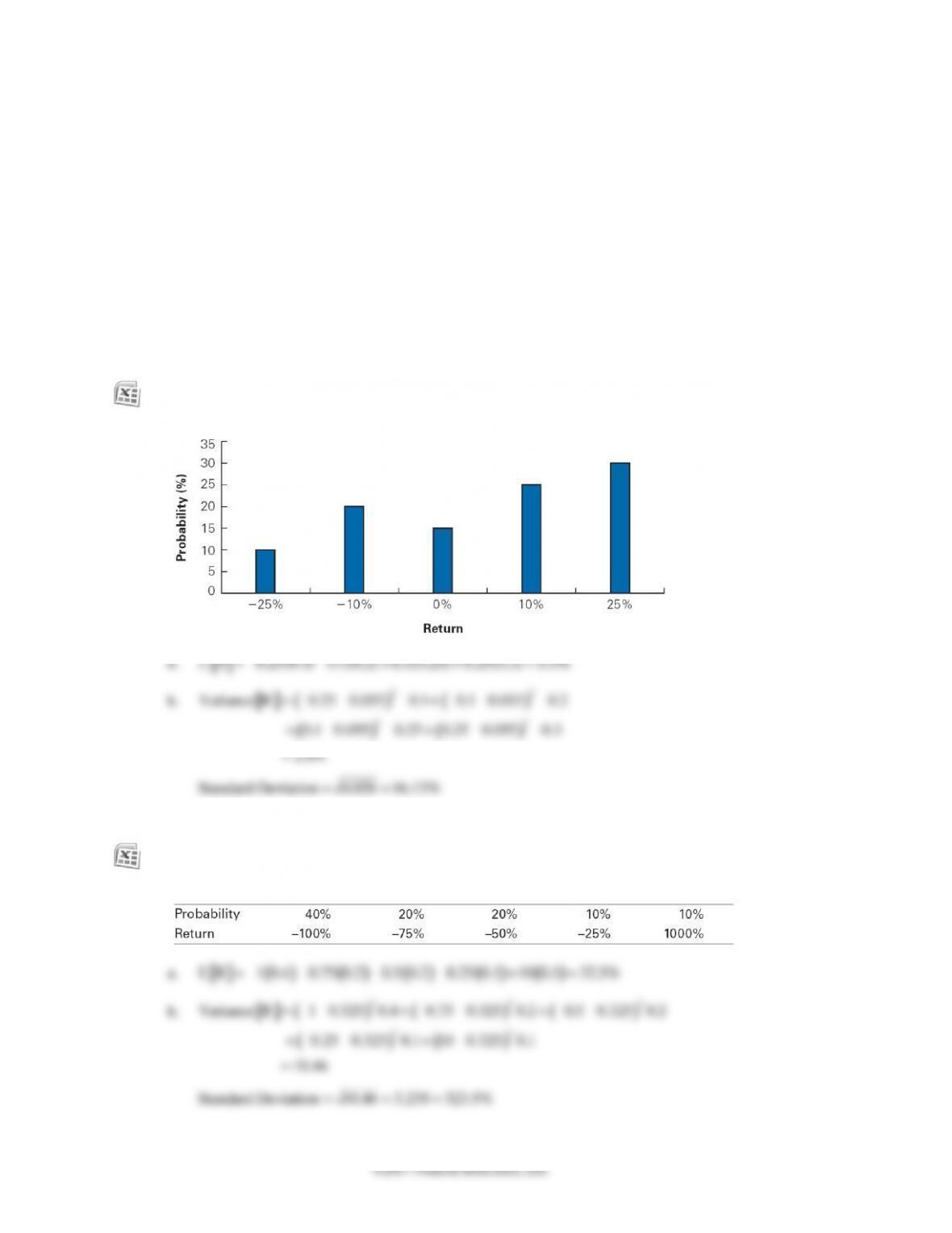
10–1. The figure below shows the one-year return distribution for RCS stock. Calculate
a. The expected return.
b. The standard deviation of the return.
10–2. The following table shows the one-year return distribution of Startup, Inc. Calculate
a. The expected return.
b. The standard deviation of the return.
Chapter 10/Capital Markets and the Pricing of Risk 145
you can use the function normdist (x,mean,volatility,1) in Excel to compute the probability
that a normally distributed variable with a given mean and volatility will fall below x.)
c. Do all the probabilities you calculated in part (b) make sense? If so, explain. If not, can you
identify the reason?
Investment
Return
Volatility
(Standard
Deviation)
Average
Annual
Return
Standard
Error
Lower
Bound
Confidence
Interval
Upper
Bound
Confidence
Interval
Part b
answer
Small
stocks
39.20%
18.70%
4.23%
10.24%
27.16%
27.27%
72.73%
S&P 500
20.30%
11.70%
2.19%
7.32%
16.08%
20.54%
79.46%
Corporate
bonds
7.00%
6.60%
0.75%
5.10%
8.10%
4.87%
95.13%
Treasury
bills
3.10%
3.90%
0.33%
2.93%
4.27%
0.20%
99.80%
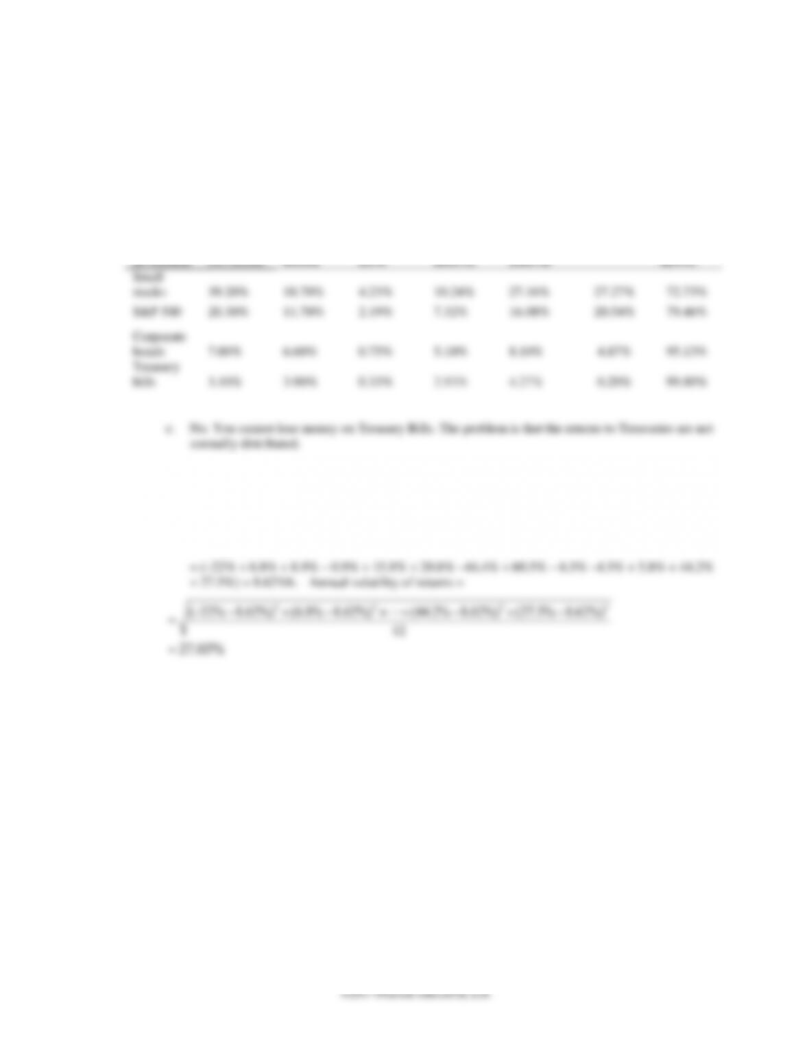
c. No. You cannot lose money on Treasury Bills. The problem is that the returns to Treasuries are not
normally distributed.
10-9. Using the data in Table 10.2,
a. What was the average annual return of Microsoft stock from 2002–2014?
b. What was the annual volatility for Microsoft stock from 2002–2014?
a. Average annual return
10–10. Using the data in Table 10.2,
a. What was the average dividend yield for the SP500 from 2002–2011?
b. What was the volatility of the dividend yield?
c. What was the average annual return of the SP500 from 2002–2011 excluding dividends (i.e.,
from capital gains only)?
d. What was the volatility of the S&P 500 returns from capital gains?
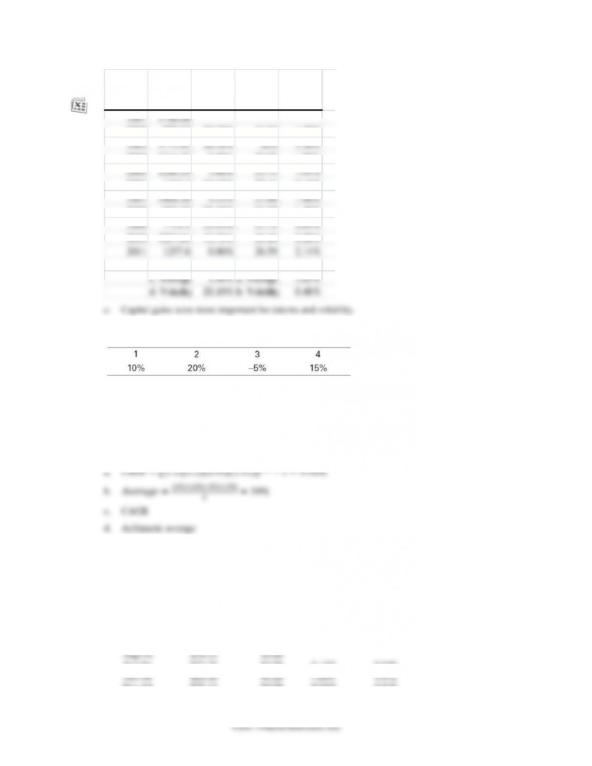
e. Were dividends or capital gains a more important component of the S&P 500’s average
returns during this period? Which were the more important source of volatility?
146 Berk/DeMarzo, Corporate Finance, Fourth Edition, Global Edition
Year End
S&P 500
Index
Capital
Gains
Return
Dividend
s Paid
Dividend
Yield
2001 1148.08
2002 879.82 –23.37% 14.53 1.27%
2003 1111.92 26.38% 20.8 2.36%
2004 1211.92 8.99% 20.98 1.89%
2005 1248.29 3.00% 23.15 1.91%
2006 1418.3 13.62% 27.16 2.18%
2007 1468.36 3.53% 27.86 1.96%
2008 903.25 –38.49% 21.85 1.49%
2009 1115.1 23.45% 27.19 3.01%
2010 1257.64 12.78% 25.44 2.28%
2011 1257.6 0.00% 26.59 2.11%
c. Average 2.99% a. Average 2.05%
d. Volatility
20.10%
b. Volatility
0.48%
e. Capital gains were more important for returns and volatility.
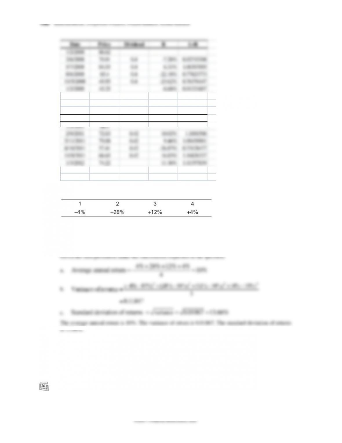
10–11. Consider an investment with the following returns over four years:
a. What is the compound annual growth rate (CAGR) for this investment over the four years?
b. What is the average annual return of the investment over the four years?
c. Which is a better measure of the investment’s past performance?
d. If the investment’s returns are independent and identically distributed, which is a better
measure of the investment’s expected return next year?
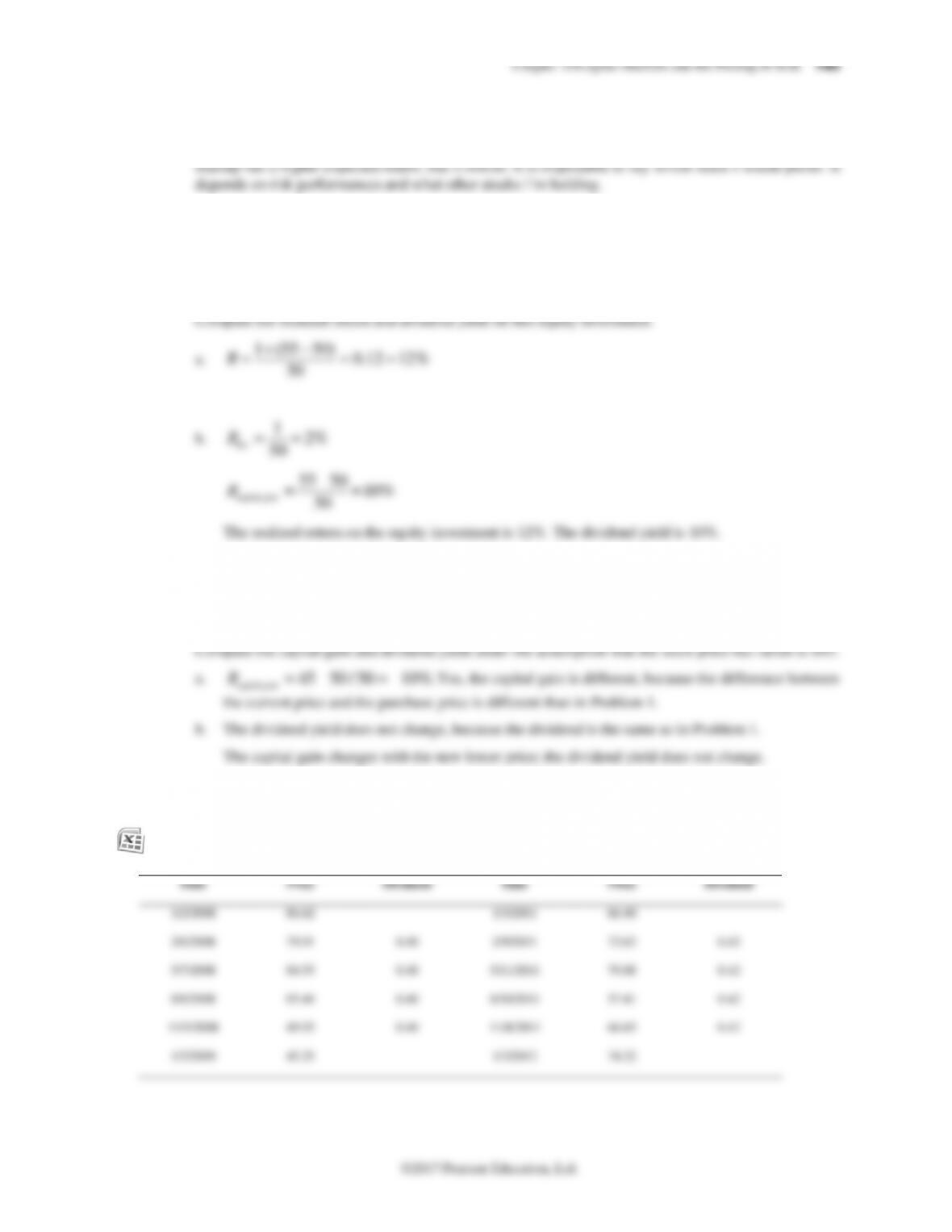
10–12. Download the spreadsheet from MyFinanceLab that contains historical monthly prices and
dividends (paid at the end of the month) for Ford Motor Company stock (Ticker: F) from August
1994 to August 1998. Calculate the realized return over this period, expressing your answer in
as an investment in Ford stock over this period).
Ford Motor Co (F)
Date
Stock Price
Dividend
Return
1+Rt
Aug-94
$29.25
$0.00
Oct–94
$29.50
$0.26
7.24%
1.072
Nov-94
$27.13
$0.00
-8.05%
0.919

Chapter 10/Capital Markets and the Pricing of Risk 147
Date
Stock Price
Dividend
Return
1+Rt
Dec–94
$27.88
$0.00
2.76%
1.028
Jan-95
$25.25
$0.26
-8.48%
0.915
Feb-95
$26.13
$0.00
3.47%
1.035
Mar–95
$26.88
$0.00
2.87%
1.029
Apr-95
$27.13
$0.31
2.08%
1.021
May–95
$29.25
$0.00
7.83%
1.078
Jun-95
$29.75
$0.00
1.71%
1.017
Jul-95
$29.00
$0.31
-1.48%
0.985
Aug-95
$30.75
$0.00
6.03%
1.060
Sep-95
$31.13
$0.00
1.22%
1.012
Oct–95
$28.75
$0.35
-6.51%
0.935
Nov-95
$28.25
$0.00
-1.74%
0.983
Dec–95
$28.88
$0.00
2.21%
1.022
Jan-96
$29.50
$0.35
3.38%
1.034
Feb-96
$31.25
$0.00
5.93%
1.059
Mar–96
$34.38
$0.00
10.00%
1.100
Apr-96
$35.88
$0.35
5.38%
1.054
May–96
$36.50
$0.00
1.74%
1.017
Jun-96
$32.38
$0.00
-11.30%
0.887
Jul-96
$32.38
$0.39
1.19%
1.012
Aug-96
$33.50
$0.00
3.47%
1.035
Sep-96
$31.25
$0.00
-6.72%
0.933
Oct–96
$31.25
$0.39
1.23%
1.012
Nov-96
$32.75
$0.00
4.80%
1.048
Dec–96
$32.25
$0.00
-1.53%
0.985
Jan-97
$32.13
$0.39
0.81%
1.008
Feb-97
$32.88
$0.00
2.33%
1.023
Mar–97
$31.38
$0.00
-4.56%
0.954
Apr-97
$34.75
$0.42
12.10%
1.121
May–97
$37.50
$0.00
7.91%
1.079
Jun-97
$38.00
$0.00
1.33%
1.013
Jul-97
$40.88
$0.42
8.67%
1.087
Aug-97
$43.00
$0.00
5.20%
1.052
Sep-97
$45.13
$0.00
4.94%
1.049
Oct–97
$43.69
$0.42
-2.25%
0.977
Nov-97
$43.00
$0.00
-1.57%
0.984
Dec–97
$48.56
$0.00
12.94%
1.129
Jan-98
$51.00
$0.42
5.88%
1.059
Feb-98
$56.56
$0.00
10.91%
1.109
Mar–98
$64.81
$0.00
14.59%
1.146
Apr-98
$45.81
$23.68
7.22%
1.072
May–98
$51.88
$0.00
13.23%
1.132
Jun-98
$59.00
$0.00
13.73%
1.137
Jul-98
$57.00
$0.42
-2.68%
0.973
Aug-98
$44.63
$0.00
-21.71%
0.783
Total Return (product of 1+R’s)
1.7102
Equivalent Monthly return = (TotalReturn)^(1/48)-1
2.10%
10–13. Using the same data as in Problem 12, compute the
a. Average monthly return over this period.
b. Monthly volatility (or standard deviation) over this period.
©2017 Pearson Education, Ltd.
10–14. Explain the difference between the average return you calculated in Problem 13(a) and the realized
return you calculated in Problem 12. Are both numbers useful? If so, explain why.
10–15. Compute the 95% confidence interval of the estimate of the average monthly return you calculated
in Problem 13(a).
Month
Stock Price
Dividend
Return
Aug-98
44.625
-0.21711
Jul-98
57.000
0.420
-0.02678
Jun-98
59.000
0.13735
May–98
51.875
0.13233
Apr-98
45.813
23.680
0.07221
Mar–98
64.813
0.14586
Feb-98
56.563
0.10907
Jan-98
51.000
0.420
0.05884
Dec–97
48.563
0.12936
Nov-97
43.000
-0.01574
Oct–97
43.688
0.420
-0.02255
Sep-97
45.125
0.04942
Aug-97
43.000
0.05199
Jul-97
40.875
0.420
0.08671
Jun-97
38.000
0.01333
May–97
37.500
0.07914
Apr-97
34.750
0.420
0.12096
Mar–97
31.375
-0.04563
Feb-97
32.875
0.02335
Jan-97
32.125
0.385
0.00806
Dec–96
32.250
-0.01527
Nov-96
32.750
0.04800
Oct–96
31.250
0.385
0.01232
Sep-96
31.250
-0.06716
Aug-96
33.500
0.03475
Jul-96
32.375
0.385
0.01189
Jun-96
32.375
-0.11301
May–96
36.500
0.01742
Apr-96
35.875
0.350
0.05382
Mar–96
34.375
0.10000
Feb-96
31.250
0.05932
Jan-96
29.500
0.350
0.03377
Dec–95
28.875
0.02212
Nov-95
28.250
-0.01739
Oct–95
28.750
0.350
-0.06506
Sep-95
31.125
0.01220
Aug-95
30.750
0.06034
Jul-95
29.000
0.310
-0.01479
Jun-95
29.750
0.01709
Chapter 10/Capital Markets and the Pricing of Risk 149
Month
Stock Price
Dividend
Return
May–95
29.250
0.07834
Apr-95
27.125
0.310
0.02084
Mar–95
26.875
0.02871
Feb-95
26.125
0.03465
Jan-95
25.250
0.260
-0.08484
Dec–94
27.875
0.02765
Nov-94
27.125
-0.08051
Oct–94
29.500
0.260
0.07243
Sep-94
27.750
-0.05128
Aug-94
29.250
Average Monthly Return
2.35%
Std Dev of Monthly Return
7.04%
Std Error of Estimate = (Std Dev)/sqrt(36) =
1.02%
95% Confidence Interval of average monthly return
0.31%
4.38%
10–16. How does the relationship between the average return and the historical volatility of individual
stocks differ from the relationship between the average return and the historical volatility of large,
well-diversified portfolios?
10-17. Download the spreadsheet from MyFinanceLab containing the data for Figure 10.1.
a. Compute the average return for each of the assets from 1929 to 1940 (The Great Depression).
b. Compute the variance and standard deviation for each of the assets from 1929 to 1940.
c. Which asset was riskiest during the Great Depression? How does that fit with your intuition?
a/b.
S&P 500
Small Stocks
Corp Bonds
World
Portfolio
Treasury Bills
CPI
Average
2.55%
15.65%
5.35%
2.94%
0.83%
-1.48%
Variance:
0.10179
0.50460
0.00129
0.06968
0.00020
0.00221
Standard
deviation:
31.90%
71.03%
3.59%
26.40%
1.40%
4.70%
Evaluate:
c. The riskiest assets were the small stocks. Intuition tells us that this asset class would be the riskiest.
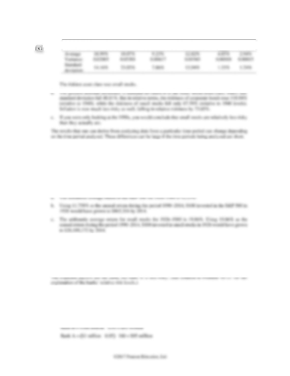
10–18. Using the data from Problem 17, repeat your analysis over the 1990s.
a. Which asset was riskiest?
b. Compare the standard deviations of the assets in the 1990s to their standard deviations in the
Great Depression. Which had the greatest difference between the two periods?
c. If you only had information about the 1990s, what would you conclude about the relative risk
of investing in small stocks?
150 Berk/DeMarzo, Corporate Finance, Fourth Edition, Global Edition
a. Using Excel:
S&P 500
Small Stocks
Corp Bonds
World Portfolio
Treasury
Bills
CPI
Average
18.99%
10.07%
9.23%
12.82%
4.85%
2.94%
Variance:
0.02005
0.05301
0.00617
0.01943
0.00018
0.00015
Standard
deviation:
14.16%
23.02%
7.86%
13.94%
1.33%
1.24%
10–19. What if the last two decades had been “normal”? Download the spreadsheet from MyFinanceLab
containing the data for Figure 10.1.
a. Calculate the arithmetic average return on the S&P 500 from 1926 to 1989.
b. Assuming that the S&P 500 had simply continued to earn the average return from (a),
calculate the amount that $100 invested at the end of 1925 would have grown to by the end of
2014.
c. Do the same for small stocks.
10–20. Consider two local banks. Bank A has 100 loans outstanding, each for $1 million, that it expects
will be repaid today. Each loan has a 5% probability of default, in which case the bank is not
repaid anything. The chance of default is independent across all the loans. Bank B has only one
loan of $100 million outstanding, which it also expects will be repaid today. It also has a 5%
probability of not being repaid. Explain the difference between the type of risk each bank faces.
Which bank faces less risk? Why?
10–21. Using the data in Problem 20, calculate
a. The expected overall payoff of each bank.
b. The standard deviation of the overall payoff of each bank.
a. Expected payoff is the same for both banks
Bank B $100 million 0.95 $95 million= ´ =
( )
Bank A $1 million 0.95 100 $95 million= ´ ´ =
Chapter 10/Capital Markets and the Pricing of Risk 151
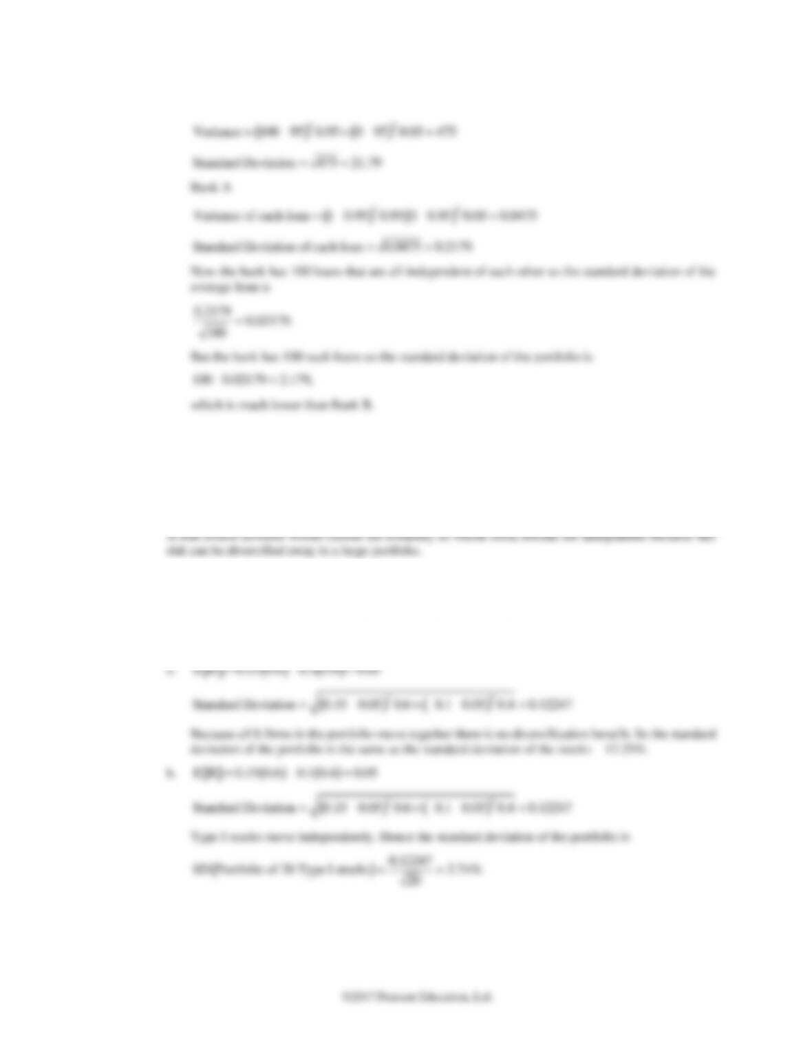
b. Bank B
( ) ( )
2 2
Variance 100 95 0.95 0 95 0.05 475= – + – =
Standard Deviation 475 21.79= =
Bank A
( ) ( )
2 2
Variance of each loan 1 0.95 0.95 0 0.95 0.05 0.0475= – – =
Standard Deviation of each loan 0.0475 0.2179= =
Now the bank has 100 loans that are all independent of each other so the standard deviation of the
average loan is
0.2179 0.02179.
100 =
But the bank has 100 such loans so the standard deviation of the portfolio is
100 0.02179 2.179,´ =
which is much lower than Bank B.
10–22. Consider the following two, completely separate, economies. The expected return and volatility of
all stocks in both economies is the same. In the first economy, all stocks move together—in good
times all prices rise together and in bad times they all fall together. In the second economy, stock
returns are independent—one stock increasing in price has no effect on the prices of other stocks.
Assuming you are risk-averse and you could choose one of the two economies in which to invest,
which one would you choose? Explain.
10–23. Consider an economy with two types of firms, S and I. S firms all move together. I firms move
independently. For both types of firms, there is a 60% probability that the firms will have a 15%
return and a 40% probability that the firms will have a −10% return. What is the volatility
(standard deviation) of a portfolio that consists of an equal investment in 20 firms of (a) type S,
and (b) type I?
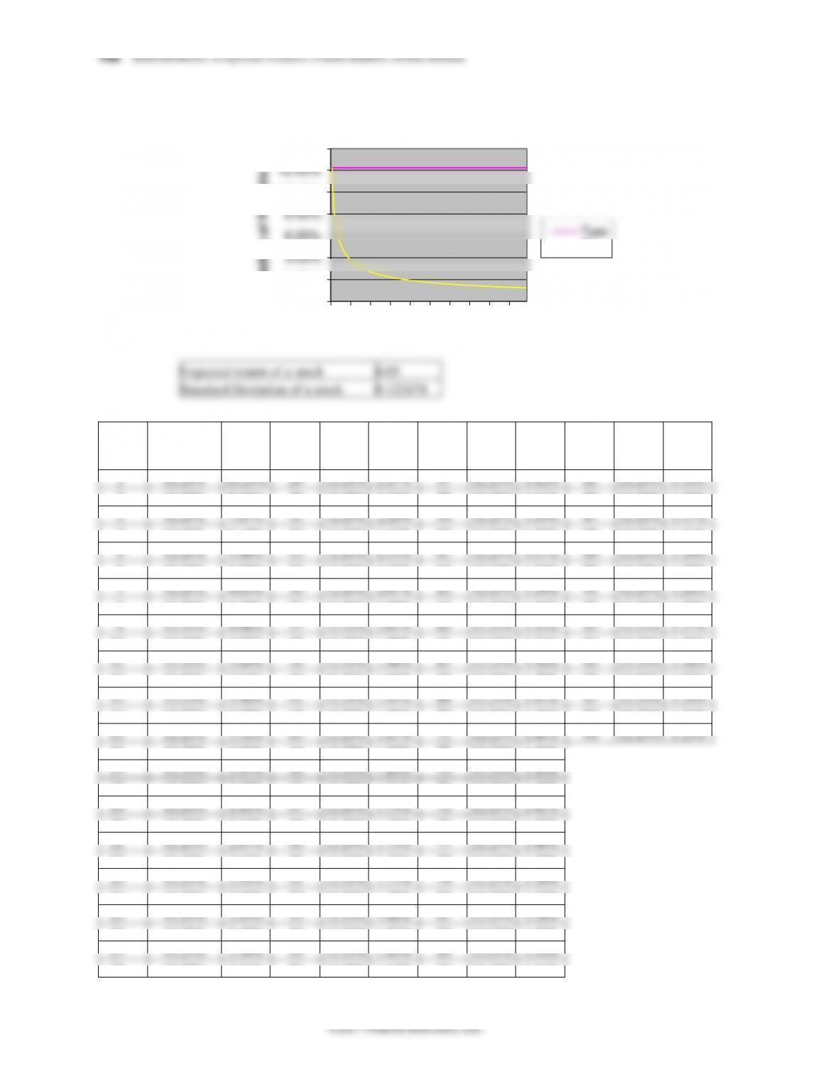
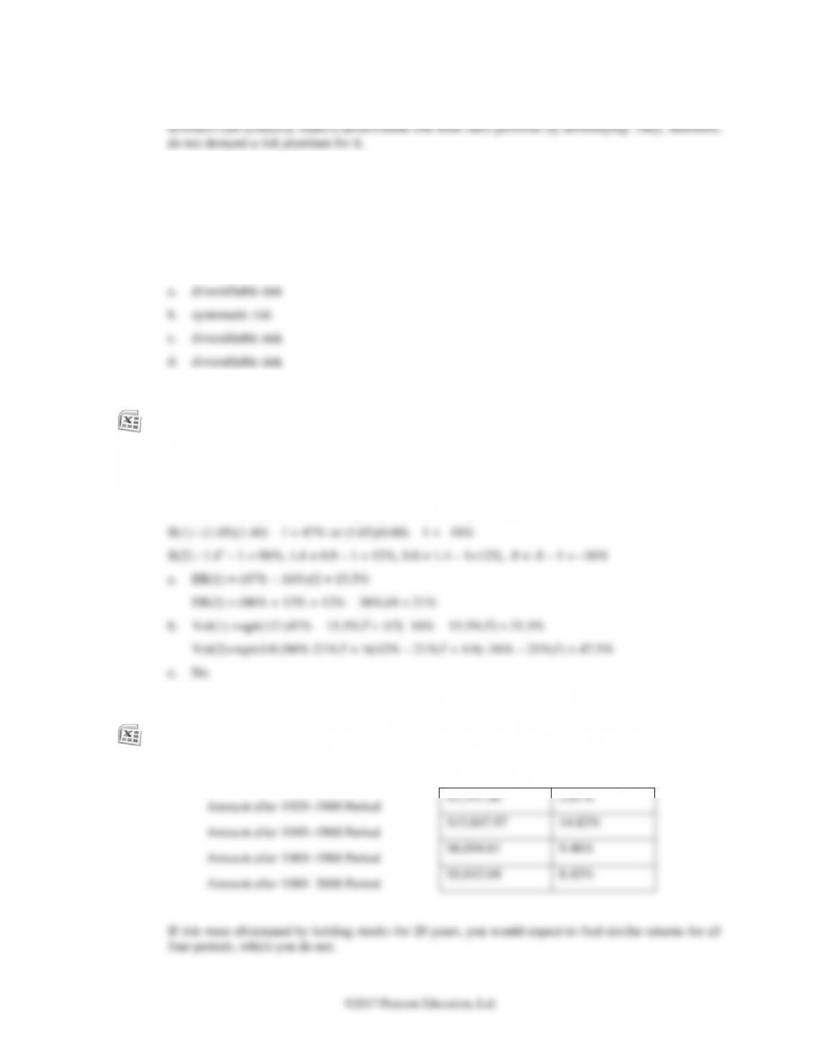
20
Chapter 10/Capital Markets and the Pricing of Risk 153
10–25. Explain why the risk premium of a stock does not depend on its diversifiable risk.
10–26. Identify each of the following risks as most likely to be systematic risk or diversifiable risk:
a. The risk that your main production plant is shut down due to a tornado.
b. The risk that the economy slows, decreasing demand for your firm’s products.
c. The risk that your best employees will be hired away.
d. The risk that the new product you expect your R&D division to produce will not materialize.
10–27. Suppose the risk–free interest rate is 5%, and the stock market will return either 40% or −20%
each year, with each outcome equally likely. Compare the following two investment strategies: (1)
invest for one year in the risk-free investment, and one year in the market, or (2) invest for both
years in the market.
a. Which strategy has the highest expected final payoff?
b. Which strategy has the highest standard deviation for the final payoff?
c. Does holding stocks for a longer period decrease your risk?
10–28. Download the spreadsheet from MyFinanceLab containing the realized return of the S&P 500
from 1929–2008. Starting in 1929, divide the sample into four periods of 20 years each. For each
20-year period, calculate the final amount an investor would have earned given a $1000 initial
investment. Also express your answer as an annualized return. If risk were eliminated by holding
stocks for 20 years, what would you expect to find? What can you conclude about long-run
diversification?
Amount after 1929–1948 Period
$1,741.26
2.81%
Amount after 1949–1968 Period
$15,847.97
14.82%
Amount after 1969–1988 Period
$6,094.61
9.46%
Amount after 1989–2008 Period
$5,043.04
8.43%
If risk were eliminated by holding stocks for 20 years, you would expect to find similar returns for all
four periods, which you do not.
Chapter 10/Capital Markets and the Pricing of Risk 155
b. i. Use the beta you calculated for the stock in Problem 33(b) to estimate its expected return.
ii. How does this compare with the stock’s actual expected return?
10–35. Suppose the market risk premium is 5% and the risk-free interest rate is 4%. Using the data in
Table 10.6, calculate the expected return of investing in
a. Starbucks’ stock.
b. Hershey’s stock.
c. Autodesk’s stock.
10–36. Given the results to Problem 35, why don’t all investors hold Autodesk’s stock rather than
Hershey’s stock?
10–37. Suppose the market risk premium is 6.5% and the risk-free interest rate is 5%. Calculate the cost
of capital of investing in a project with a beta of 1.2.
[ ]
( ) ( )
Cost of Capital E R 5 1.2 6.5 12.8%
f m f
r r
b
= + – = + =
10–38. State whether each of the following is inconsistent with an efficient capital market, the CAPM, or
both:
a. A security with only diversifiable risk has an expected return that exceeds the risk-free interest
rate.
b. A security with a beta of 1 had a return last year of 15% when the market had a return of 9%.
c. Small stocks with a beta of 1.5 tend to have higher returns on average than large stocks with
a beta of 1.5.