
Algorithms: Sequential, Parallel and Distributed 6-1
Chapter 6
Probability and the Average Behavior of Algorithms
At a Glance
Table of Contents
• Overview
• Objectives
• Instructor Notes
• Solutions to Selected Exercises
Algorithms: Sequential, Parallel and Distributed 6-2
Lecture Notes
Overview
In Chapter 6 we discuss the probabilistic analysis of algorithms. We begin by giving a formal
definition of the notion of average complexity in terms of the expected value of the number τ of
basic operations performed by an algorithm for an input of size n. We then given five
formulations for the average complexity A(n), and discuss conditions under which the various
formulations are appropriate. We illustrate these ideas by analyzing the average complexity of
the algorithms LinearSearch, InsertionSort, QuickSort, MaxMin2, BinarySearch,
SearchBinSrchTree, and LinkOrdLinSrch.
Chapter Objectives
After completing the chapter the student will know:
• The formal definition of the average complexity A(n) of an algorithms in terms of the
expected value of the number of basic operations performed
• Various equivalent formulations of A(n) and conditions determining which of the
Instructor Notes
The material in this chapter is somewhat more sophisticated than the material in the previous
chapters. For example, the analysis of the algorithm LinkOrdLinSrch is fairly involved and the
instructor may wish to omit it depending on the sophistication and background of the students.
On the other hand, the analysis of LinkOrdLinSrch is particularly illustrative of the various
concepts used in determining average behavior. Appendix E provides background material for
the basic probability theory that is used in the definitions and the average analysis of the
algorithms in this chapter. The student might be familiar with this material from taking a first
Algorithms: Sequential, Parallel and Distributed 6-3
Solutions to Selected Exercises
Section 6.1 Expectation and Average Complexity
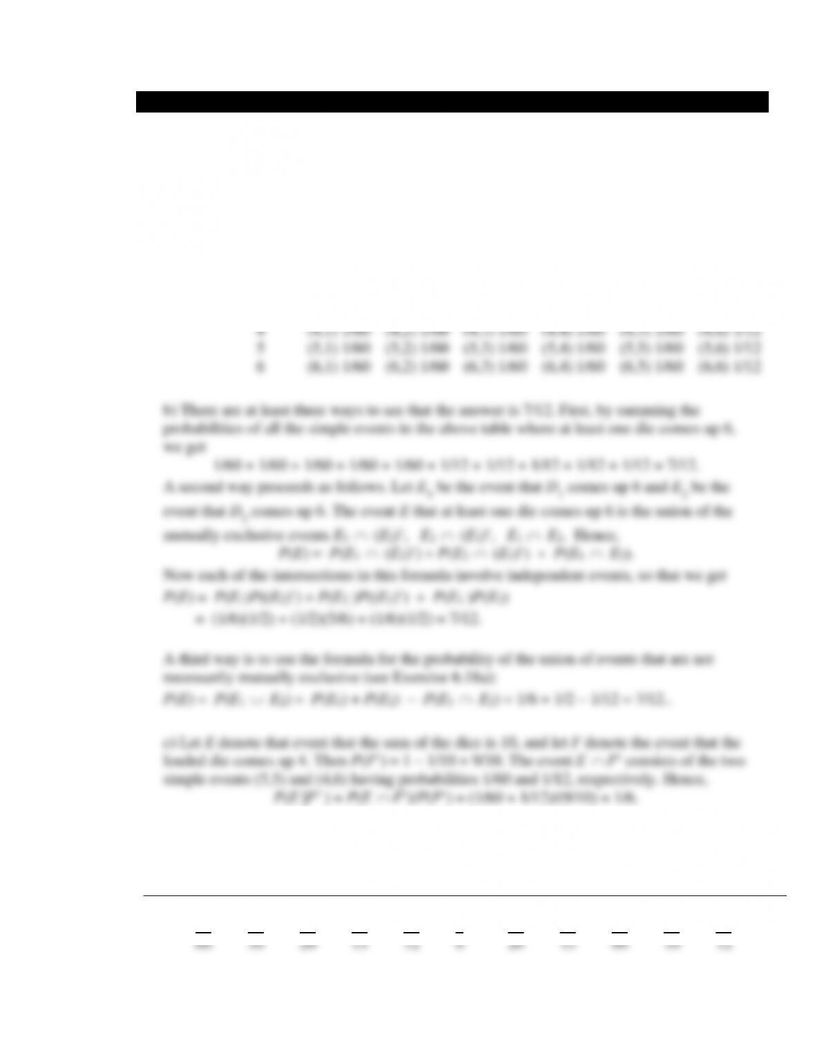
6.1 The following table shows the probabilities of the indicated outcomes.
D2
1
2
3
4
5
6
D1
1
(1,1) 1/60
(1,2) 1/60
(1,3) 1/60
(1,4) 1/60
(1,5) 1/60
(1,6) 1/12
2
(2,1) 1/60
(2,2) 1/60
(2,3) 1/60
(2,4) 1/60
(2,5) 1/60
(2,6) 1/12
3
(3,1) 1/60
(3,2) 1/60
(3,3) 1/60
(3,4) 1/60
(3,5) 1/60
(3,6) 1/12
4
(4,1) 1/60
(4,2) 1/60
(4,3) 1/60
(4,4) 1/60
(4,5) 1/60
(4,6) 1/12
5
(5,1) 1/60
(5,2) 1/60
(5,3) 1/60
(5,4) 1/60
(5,5) 1/60
(5,6) 1/12
6
(6,1) 1/60
(6,2) 1/60
(6,3) 1/60
(6,4) 1/60
(6,5) 1/60
(6,6) 1/12
6.2 a)
Probabilities pj for the sum j of the two dice from Ex. 6.1
j
2
3
4
5
6
7
8
9
10
11
12
pj
1
60
1
30
1
20
1
15
1
12
1
6
3
20
2
15
7
60
1
10
1
12
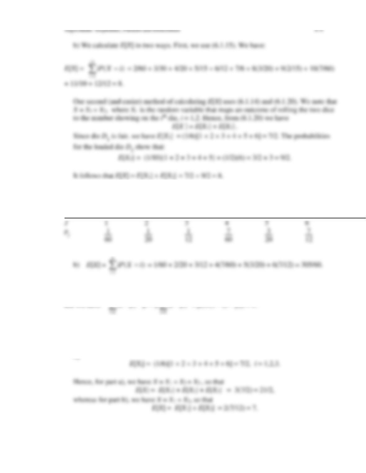
2
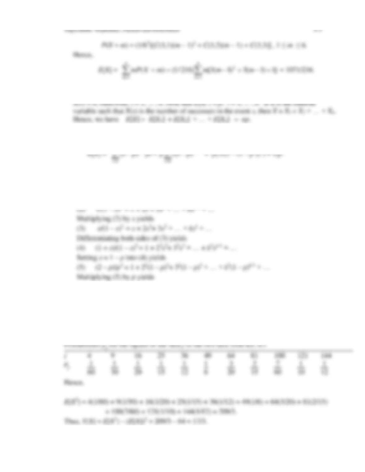
6.3 a)
Probabilities pj for the maximum j
of the two dice from Ex. 6.1
J
1
2
3
4
5
6
pj
1
60
1
20
1
12
7
60
3
20
7
12
=
6
1
i
6.4 We have
=
=
−−=−
01
1)1()1(
i
i
i
ipppp
= p(1/(1 – (1 – p)) = 1.
6.5 For parts a) and b), suppose we let Xi be the random variable that maps an outcome of
rolling the three dice to the number showing on the ith die, i = 1,2,3. Then, since the outcome
of die i is independent of the outcomes of the other two dice, the expectation of Xi is given
by
c) Now for 1 m 6, by noting that the maximum value of r1, r2, r3 can occur at one,two,
or three of the dice, respectively, we have
1
1
mm
6.6 Let Xi be the random variable such that X(s) = 1 if the event s had a success in the ith trial,
6.7 We have
−
−−=−
1
1)1()1(
i
ipippip
have the following table for pj = P((max{r1 , r2 })2 = j)
Probabilities pj for the square of the maximum j
of the two dice from Ex. 6.1
J
1
4
9
16
25
36
pj
1
60
1
20
1
12
7
60
3
20
7
12
Hence, E[X2] = 1(1/60) + 4(1/20) + 9(1/12) + 16(7/60) + 25(3/20) + 36(7/12) = 1655/60.
Thus, V[X] = E[X2] – (E[X])2 = 1655/60 – (305/60)2 = 6275/(60)2 = 251/144.
6.10 a) Consider the random variable X = r1 + r2 + r3. To compute V[X], it is convenient to
note that r1, r2, r3 are pairwise independent variables, so that V[r1 + r2 + r3] = V[r1] + V[r2] +
c) For X = max{r1, r2, r3}, we use the result from Exercise 6.5, so that
E[X] =
]1)1(3)1(3[)216/1()( 6
1
2
6
1
+−+−== ==
mmmmXmP
mm
= 1071/216,
22
6
22 +−+−== ==
6.11 a) We first show that if X and Y are independent random variables, then E[XY] = E[X]E[Y].
We have
======
yxyx
yYPxXxyPyYyPxXxPYEXE
,
))()())(())((][][
j
nji iXX
12
= E[(X1)2] + E[(X2)2] + … + E[(Xn)2] +
][2
1j
nji iXXE
– ((E[X1])2 + (E[X2])2+ … + (E[Xn])2 +
][][2
1j
nji iXEXE
)
][][2
1j
nji iXEXE
= E[(X1)2] + E[(X2)2] + … + E[(Xn)2] – ((E[X1])2 + (E[X2])2 + … + (E[Xn])2)
= E[(X1)2] – (E[X1])2 + E[(X2)2] – (E[X2])2 + … + E[(Xn)2] – (E[Xn])2
= V[X1] + V[X2] + … + V[Xn].
b) Let Xi be the random variable such that X(s) = 1 if the event s had a success in the ith trial,
X(s) = 0, otherwise, i = 1, … , n. Note that E[(Xi)2] = E[Xi] = p, i = 1, … , n. Hence, V[Xi] =
.
6.12 Given P as defined in Proposition E.1.1, we have
1.
==
SsEs
sPsPEP 1})({})({)(
.
Ss
3.
=
=
=++== n
ii
EsEsEEs
n
iiEPsPsPsPEP
nn 1…
1
)(})({…})({})({)(
11
.
6.13 We have
===
SsSs
XcEsPsXcsPscXcXE][)()()()(][
.
6.14 Defining the function
nippinCiXPiP iin ,...,0,)1)(,()()( =−=== −
,
we show that P is a probability distribution on {0,1, … , n} by using Proposition E.1.1. It is
=
−
=
==+−=−= n
i
nniin
n
i
ppppinCiP
00
11))1(()1)(,()(
using the Binomial Theorem.
Hence, the conditions of Proposition E.1.1 are satisfied, so the P is a probability distribution
on {0,1, … , n}.
6.15 That PF is a probability distribution on F follows from Proposition E.1.1 and the fact that
1)(/)()(/))(()(/)()( ====
FPFPFPsPFPsPsP
Fs F
FsFs F
6.16 If X is a random variable on the (discrete) sample space S, then we have
−
== XX SxSx xXPxf ))(()( 1
P(S) = 1.
(1) P(A
Bc) = P(A) – P(A
B).
Similarly,
(2) P(Ac
B) = P(B) – P(A
B).
b) For n sets A1, … , An, we have
= P(A1
…
An-1) + P(An) – P((A1
An)
…
(An-1
An))
=
…)()( 11
1
1+− −
−
=j
nji i
n
iiAAPAP
1
+−++−
n
kAAPAAP
1
−
n
6.22 a)
procedure InsertionSortRec(L[0:n – 1], m) recursive
Input: L[0:n – 1] (a list of size n), m (integer)
Output: L[0:m – 1] sorted in increasing order (called initially with m = n)
if m > 1 then
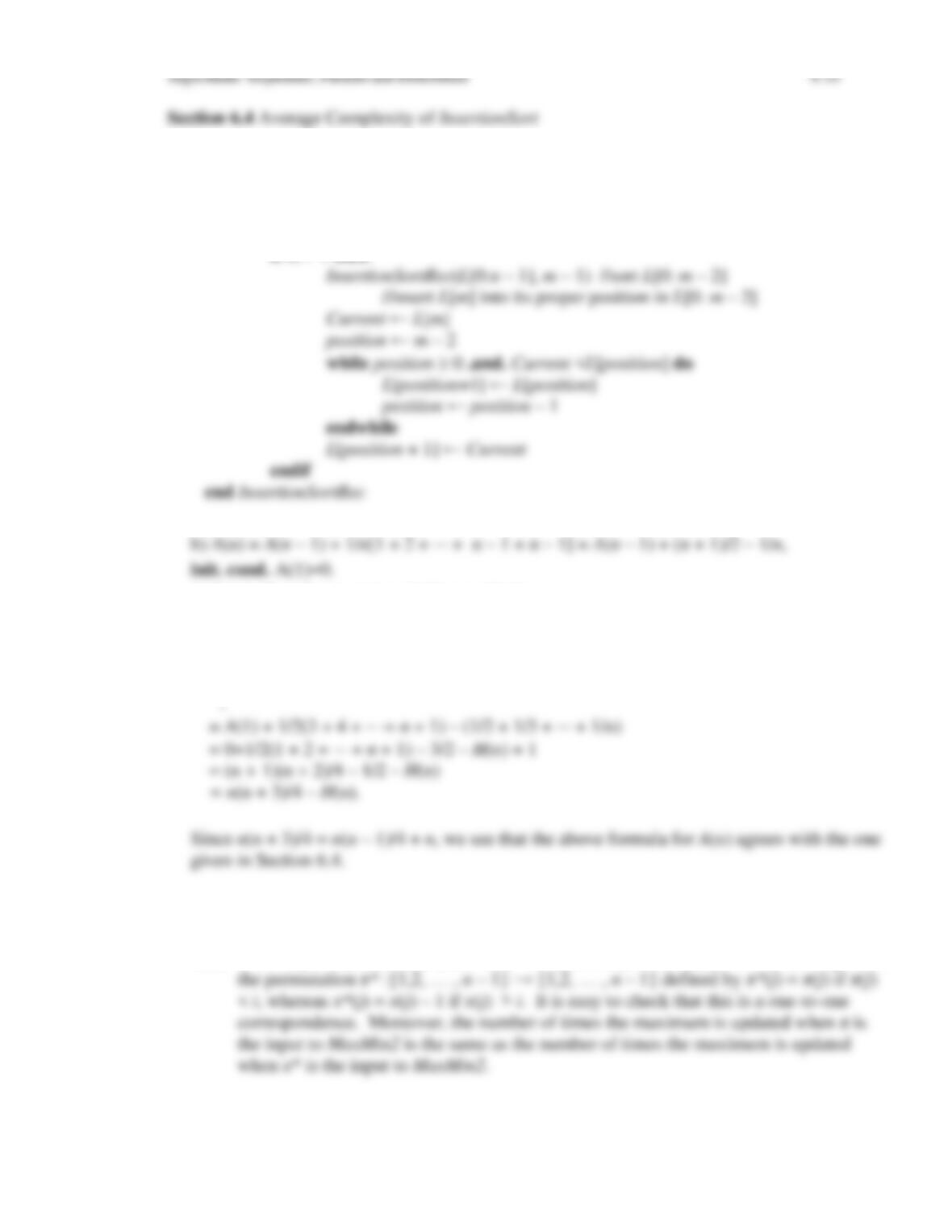
c) Unwinding the recurrence in b), we obtain
A(n) = A(n – 1) + (n + 1)/2 – 1/n
= A(n – 2) + n/2 + (n + 1)/2 – 1/(n – 1) – 1/n
Section 6.7 Average Complexity of MaxMin2
6.25 Given a permutation π : {1,2, … , n}→ {1,2, … , n}, where π(n) = i ≠ n, we map π to
Section 6.7 Average Complexity of BinarySearch and SearchBinSrchTree
6.27 Using the same argument for the implicit binary search tree that was used to establish
formula (6.7.2) for the average behavior of BinarySearch, we have for an explicit binary
search tree
A(T,n)
pTLPL
n
np
n
p
n
p
TLPL
n
p
nTLPL
n
p
−
+
−
=
+
−
+
−
+−
=
)(
1
/1
1
1
)(
1
1
))((
6.28 We assume that we compute the average behavior by inputting all permutations I n
of {1,2, … , n} and building the binary search trees associated with each permutation. As
usual, we assume all permutations are equally likely. It follows that we need to compute
the expected number of comparisons made when building a binary search tree. We first
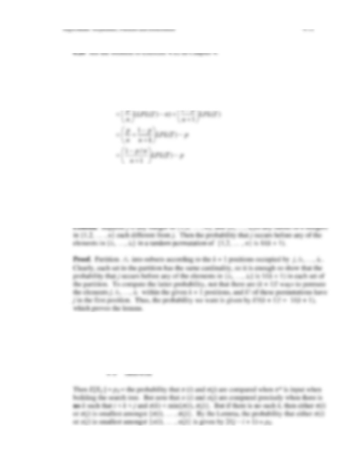
prove the following lemma.
Given a permutation π*, associate with π* the permutation π, where π(i) is the position of i
in the permutation π*. For example, if π* is the permutation 3,2,5,1,4, then
π is the permutation 4,2,1,5,3. For 1 ≤ i < j ≤ n, consider the (indicator) random variable Xij
defined on I n defined as follows.
Xij (π*) = 1 if π(i) and π(j) are compared when π* is input when building the search tree

Algorithms: Sequential, Parallel and Distributed 6-12
Section 6.8 Searching a Link-Ordered List
6.29 When searching for the maximum element in the link-order list, we first do n/2 index
6.31 Let A denote the event that X occurs on the list, and B the complementary event. Then
P(A) = p, and P(B) = 1 – p. Then by formula E.4.5 of Appendix E,