Algorithms: Sequential, Parallel and Distributed 3-1
Chapter 3
Mathematical Tools for Algorithm Analysis
At a Glance
Table of Contents
• Overview
• Objectives
• Instructor Notes
• Solutions to Selected Exercises

Algorithms: Sequential, Parallel and Distributed 3-2
Lecture Notes
Overview
In Chapter 3 we establish fundamental concepts relating to asymptotic growth rates of
functions. In particular, we define the complexity classes O(n), Θ(n), and Ω(n), and establish
various results that help in determining membership in these classes. We also obtain order
formulas for three important series—sum of powers, sum of logarithms and the harmonic
series.
In Chapter 3 we also provide the student with a glimpse of lower bound theory. In
particular we show that any adjacent-key comparison-based sorting algorithm must perform at
least n(n+1)/2 comparisons in the worst case and n(n+1)/4 comparisons on average under the
It is important to establish correctness of an algorithm. In this chapter we discuss the how
mathematical induction can be applied as a primary tool for establishing correctness. For
recursive algorithms, induction on the input size is usually the relevant tool. For algorithms
involving loops, the most relevant tool is establishing loop invariants using induction.
Chapter Objectives

recurrence relation, and for solving the recurrence relation to determine the order (or
perhaps exact nature) of this complexity
• The technique of establishing correctness of an algorithm using mathematical induction –
induction on the input size for recursive algorithms and establishing loop invariants for
algorithms involving loops.
Instructor Notes
Even though students may have been exposed to the classes O(f(n)), Θ(f(n)), and Ω(f(n)), they
may have only a hazy idea of what these classes mean, so that it might be advantageous to
carefully review these concepts. In any case, these classes are the standard method of
measuring asymptotic growth in algorithm analysis, and will be used throughout the text.
When analyzing algorithms it is often convenient to make assumptions about the input size n,
for example, that n is a power of 2, and we make such assumptions throughout the text. These
assumptions often give a simple recurrence relation for the complexity of the algorithm. It then
becomes important to interpolate the behavior of the algorithm between, say, the powers of 2.
Solutions to Selected Exercises
Section 3.1 Asymptotic Behavior of Functions
3.1 a) (1)1 100,000,000 (1,000,000,000)1.
3.5a)
2/1
/)(ln2
/11
lim
ln2
lim
)ln2/()(
lim 2
2
23
3
2
3
=
+
+
=
+
+
=
++
→→→ nn
n
nnn
nn
n
nnnn
nnn
(using
3.7 In this problem it is convenient to use that fact that if
=
→ ))(ln(
))(ln(
lim ng
nf
n
, then
=
→ )(
)(
lim ng
nf
n
(the converse is, of course, not generally true).
k
Formatted: Portuguese (Brazil)
Field Code Changed
1
)5ln)8/15((12
)2/25(12
lim
)4/5()4/15(ln)8/15(12
)2/25(12
lim 2/1
2/3
2/12/12/1
2/3
=
++
−+
=
+++
−+
=−
−
→
−−−
−
→ nn
n
nnnn
n
nn
n1/2 =lim
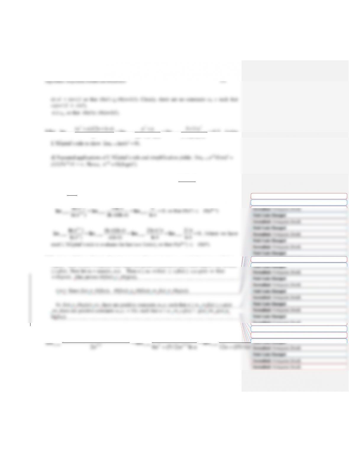
3.14 a) Suppose f(n) = aknk + ak-1nk-1 + … + a0 is a polynomial of degree k. Then by the
binomial theorem, f(n) = aknk + bk-1nk-1 + … + b0 for appropriate coefficients bk-1, …, b0.
3.15 Differentiating P(n) k times yields a constant. Differentiating an k times yields (lna)k an.
3.17 Suppose limn→∞(f(n) /g(n)) = ∞. Then there is a positive constant n0 such that n ≥ n0
f(n)/g(n) ≥ 1. Hence, n ≥ n0
f(n) ≥ g(n)
g(n)
O(f(n)). On the other hand,
b) Let f(n) = n when n is even, and f(n) = n2 when n is odd. Let g(n) = n2 for all n. Then
Algorithms: Sequential, Parallel and Distributed 3-6
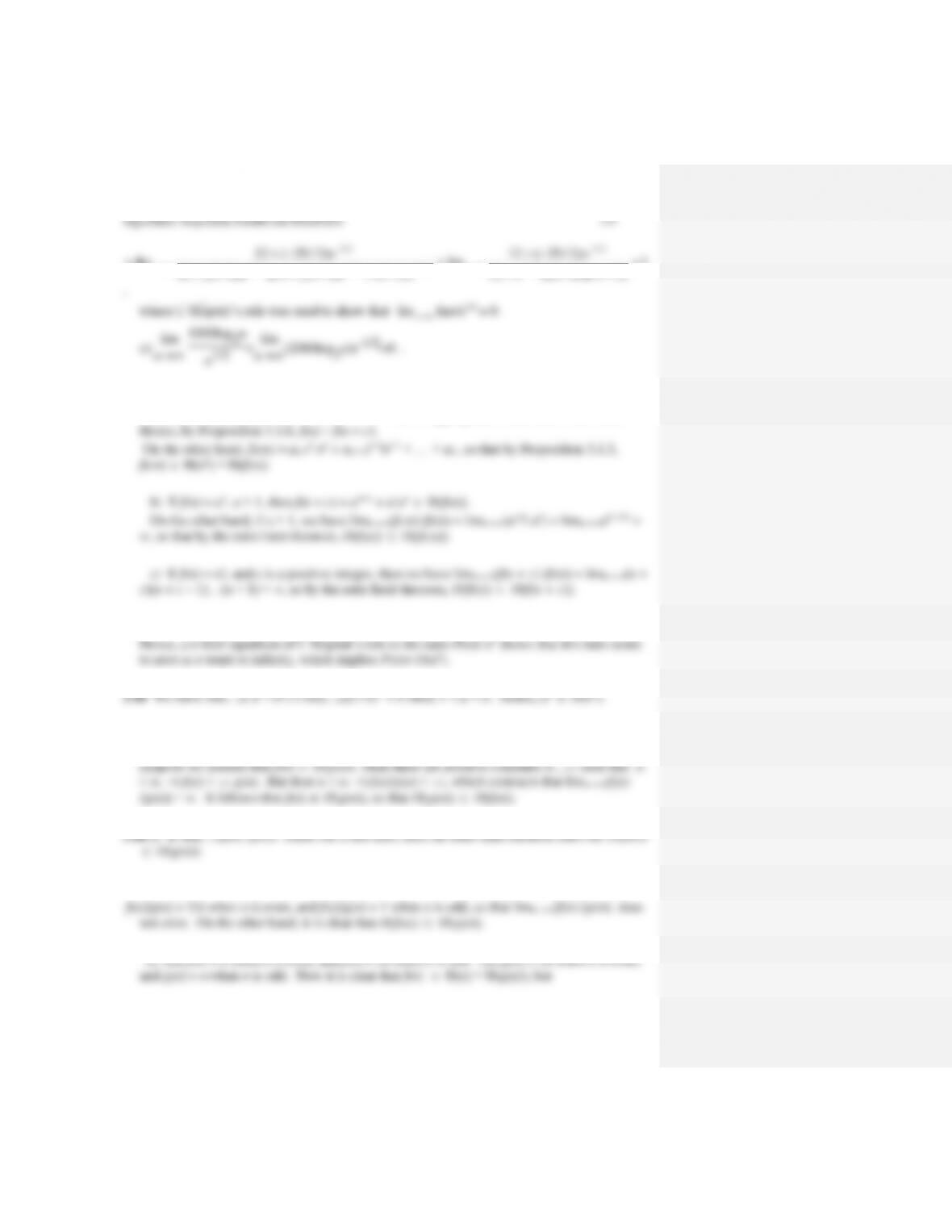
3.23 a) Reflexive Property: f K f since limn→∞(f(n) /f(n)) = 1.
3.24 Note that g(n) = n2 when n is even, and since f(n) = n3, it follows that f(n)
O(g(n)). On
3.25 A simple way to find such functions is to define them recursively. Let f(1) = g(1) = 1.
For n > 1, let f(n) = f(n – 1) + 1 if n is even, whereas f(n) = ng(n – 1) if n is odd. On the
other hand, let g(n) = g(n – 1) + 1 if n is odd, whereas g(n) = nf(n – 1 ) if n is even. Now
Section 3.2 Asymptotic Order Formulae for Three Important Series
3.26 We show that S(n) =
))(log()(log 2
1
2nni
n
i
=
.
i=1
3.28
Algorithms: Sequential, Parallel and Distributed 3-7
H(n) =1
Each grouping of terms sums to at least 1/2, so that H(n) clearly grows arbitrarily large as n
tends to infinity.
3.29 S(n,k) = 1k + 2k + … + nk ≤ nk+1, so that S(n,k) O(nk+1). On the other hand, S(n,k) ≥
3.31 We use induction on k to prove that the coefficients of nk, k 1, and nk-1 , k 2 in the
polynomial expansion of S(n,k) are 1/2 and k/12, respectively.
=
+
0
1
i
k
Using the induction hypothesis, only two terms in the above recurrence contribute to the
coefficient of nk: namely, the term involving nk in (n + 1)k (whose coefficient is C(k+1,k) = k
Now consider the coefficient of nk-1. Again, using the induction hypothesis, it follows easily
that the coefficient of nk-1 is given by:
4
)1(6
2
1
k
k
−
+
3.32 a) It follows from (3.2.1) that:
−
1
1k
Algorithms: Sequential, Parallel and Distributed 3-8
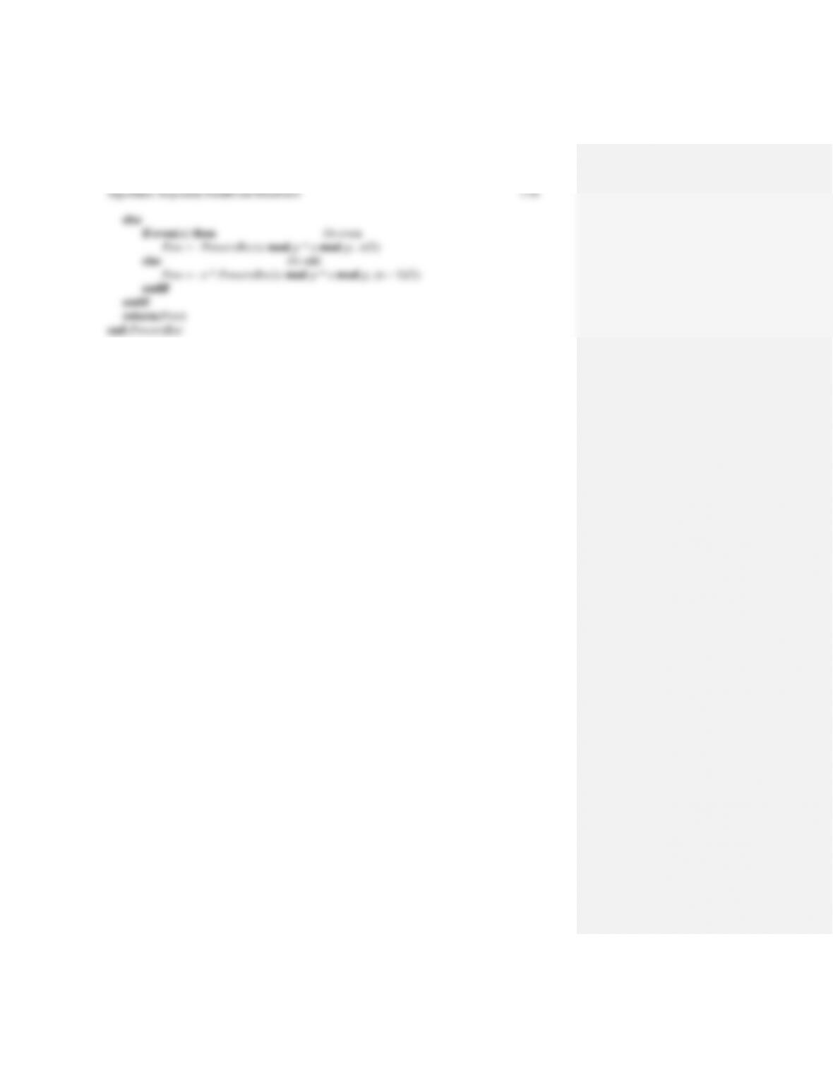
b) In the following pseudocode, BinomCoeff (n,k) is a function returning C(n,k).
endfor
for m ← 1 to k do
for j ← 1 to m do //Compute B[j, m]
Sum ← BinomCoeff(m+1, j)
for i ← j – 1 to m – 1 do
end Bernoulli
c) In the following pseudocode, EuclidGCD is as described on p. 9 in the text. We use
rational arithmetic throughout, maintaining the rational numbers as pairs of integers. For
example, (a,b) + (c,d) = (ad + bc, bd).
procedure BernoulliCoeffRational(k, B[0:k+1, 0:k, 0:1])
for m ← 1 to k do
for j ← 1 to m do
Sum[0] ← BinomCoeff(m+1, j)
Sum[1] ← 1
for i ← j – 1 to m – 1 do
endfor
endfor
endfor
end BernoulliCoeffRational
3.33 Let S(a,d,n,k) =
=
−+
n
j
k
dja
1
))1((
. Then we have:
+
+
n
i
n
k
k
1
1
Section 3.3 Recurrence Relations for Complexity
3.34 The best case occurs when the elements in one half-list are each greater than all the
elements in the other half list. For example, this happens if the list is either increasing or
decreasing. We obtain
3.35 a) t(n) = 3t(n – 1 ) + n
t(0) = (7/4)30 – 0/2 – 3/4 = 7/4 – 3/4 = 1, so the initial condition is satisfied.
b) t(n) = 4t(n – 1 ) + 5
c) We assume that n = 3k. The initial condition t(0) = 0 and the recurrence yields t(1) = 1.
Then we have;
3.36 Applying Formula (3. 3.20) with a = 2, b = t(0) + 14 + 1 = 2, and f(n) = n4 + 1, we obtain
2
=
i
4
−++
in i
−− ++
n
inn i
41 )1(222
4
−++
n
in i
2
=
i
2
=
i
Algorithms: Sequential, Parallel and Distributed 3-12
Section 3.4 Mathematical Induction and Proving the Correctness of Algorithms
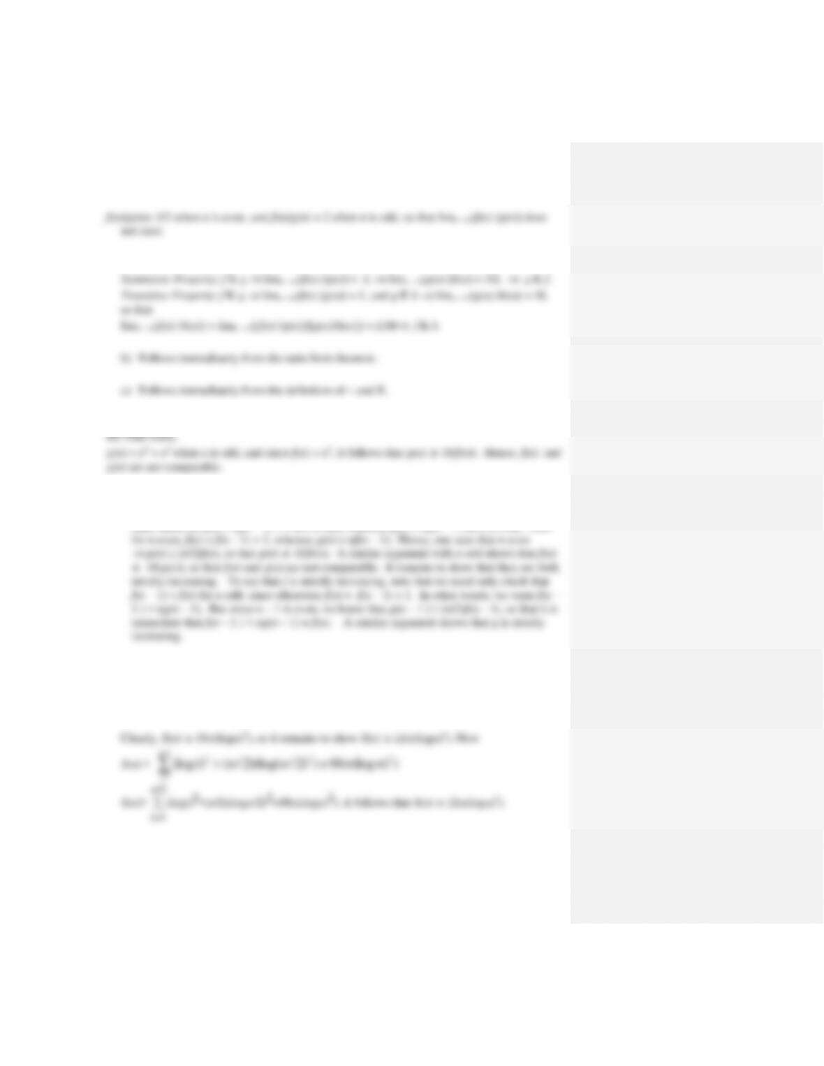
3.40 Using the binomial expansion of (1 + 1)n = 2n, we immediately obtain C(n, 0) + C(n, 1) +
… + C(n, n) = 2n.
3.41 Using the binomial expansion of (1 – 1)n = 0n = 0, we immediately obtain
C(n, 0) – C(n, 1) + … (– 1)iC(n, i) + … + (– 1)n C(n, n) = 0.
3.42 If f(n) denotes the number of regions in the plane determined by n lines, then we claim that
f(n) = 1 + n(n+1)/2.
Basis step: A line divides the plane into 2 = 1 + 1(2)/2 regions.
Induction step: Assume the formula is true for k lines. For k+1 lines, consider one of the
lines L. By induction hypothesis, the other k lines divide the plane into 1+k(k+1)/2 regions.
3.44 It is easy to prove using induction on high – low that QuickSort is correct if and only if
Partition is correct. (Note: This correction proof includes noting that the assumption L[high +
1] ≥ L[low] is maintained for the recursive calls.) We prove Partition is correct using induction
to establish the following loop invariants of its while loop.
Loop Invariants: Let x = L[low] as in the pseudocode for Partition. After k iterations of the
elements with indices between the value of moveright after the kth pass and one less than the
current value of moveright are strictly smaller than x. Thus, by induction assumption, L[i] ≤ x
for low ≤ i ≤ moveright – 1. Moveleft decreases until it reaches a value such that L[moveleft] ≤
x. In particular, all list elements with indices between the value of moveleft after the kth pass
and one less than the current value of moveleft are strictly larger than x. Thus, by induction

3.45 We prove the correctness of BubbleSort (see the solution to Exercise 3.15) by using
induction to establish the following loop invariant of its while loop.
Loop Invariant: After k passes of the while loop, 1 k n, the 1st largest, 2nd largest, … ,
kth largest elements have been properly placed in the last k index positions n – k + 1, n – k +
2, … , n. Moreover, if SwapFlag is .false. after the kth pass, then the entire list has been
3.49 We show that when GeneratePermutations is called with parameter i, it generates all
permutations of the elements T[i], …, T[n], and returns T[i:n] to its state before the
recursive call. We prove this by induction on k = n – i, i = n, …, 1.
Basis Step: k = 0. Clearly true, since GeneratePermutations simply returns, and there is
only one permutation of T[n].
Section 3.5 Establishing Lower Bounds for Problems
3.50 Suppose (π(i), π(i+1)) is an inversion, so that π(i) > π(i+1). Let π* denote the
permutation resulting from π by interchanging π(i) and π(i+1). Suppose first that j > i +1. If
3.51 Suppose there were a comparison-based algorithm for merging two lists of size n/2 to
form a list of size n and having complexity belonging to O(n1-ε). If we then use such a
merging algorithm in MergeSort, we would have a comparison-based algorithm whose
worst case would satisfy the following recurrence for n = 2k and a suitable positive constant
c:
3.53 a.
Write x = mp + r, and y = np + s, where m,n,r,s are integers and 0 ≤ r, s < p. Hence,
x mod p = r and y mod p = s. Then,
b.
function PowersRecMod(x, n) recursive