
Algorithms: Sequential, Parallel and Distributed 1-1
Chapter 22
The Fast Fourier Transform
At a Glance
Table of Contents
• Overview
• Objectives
• Instructor Notes
• Solutions to Selected Exercises
Algorithms: Sequential, Parallel and Distributed 1-2
Lecture Notes
Overview
In Chapter 22 we discuss the Discrete Fourier Transform (DFT) of a polynomial and the
celebrated Fast Fourier Transform (FFT) for computing the DFT in time O(nlogn). We
begin the chapter by defining and motivating the DFT of a polynomial P(x) with respect to
a primitive root of unity ω, denoted by DFTω(P(x)). This is followed by a discussion the
FFT algorithm for computing DFTω(P(x)) using the divide-and-conquer strategy. We then
show how the FFT can be used to multiply two polynomials whose product has size at
most n in time O(nlogn)) by transforming the problem to one of simply multiplying n
complex numbers. We finish the chapter with a discussion of how the FFT can be
implemented on the PRAM and on the Butterfly Interconnection Network.
Chapter Objectives
After completing the chapter the student will know:
• The definition of a primitive root of unity ω
• The definition of the Discrete Fourier Transform DFTω(P(x))
• The design of the FFT algorithm
Instructor Notes
When implementing the FFT on a computer, round-off errors invariably occur, since irrational
numbers are involved. To see how to deal with this issue, we refer the instructor Knuth, The
Art of Computer Programming (Vol. 2 Seminumerical Algorithms), 2nd edition, Addison
Wesley Publishing Co., Reading Mass., 1981.
Solutions to Selected Exercises
Algorithms: Sequential, Parallel and Distributed 1-3
Section 22.2 The Discrete Fourier Transform
22.1 Given P(x) = a0 + a1 x + a2 z2 + … + an-1 xn-1 , for 0 ≤ i ≤ n – 1, the value of bi given by
(22.1.2) is the dot product of the vectors [1, ωi, … , (ωi )n-1] and [a0, a1 , … , an-1]. Thus,
22.2 Let
be a primitive nth root of unity. Then we have ((ω2)n/2 = ωn = 1, so that ω2 is an
(n/2)th root of unity. Suppose is not primitive, so that there is an integer k such that 0 < k <
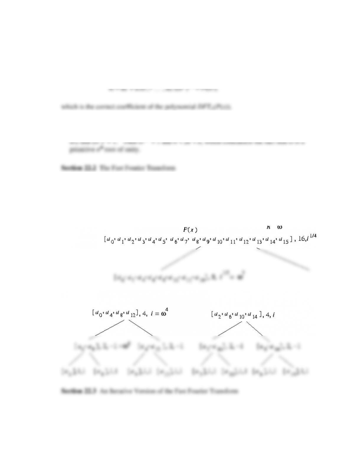
22.3 The following figure shows the root and the left subtree of the tree of recursive calls to
FFTRec with n = 16. The right subtree is obtained from the left subtree by adding one to
each subscript of the coefficients.
22.5 If n = 2k, then it is clear from the way we divide the coefficients into even- and odd-
indexed coefficients that the mapping πk:{0, …, n – 1} → {0, …, n – 1} satisfies the
relation:
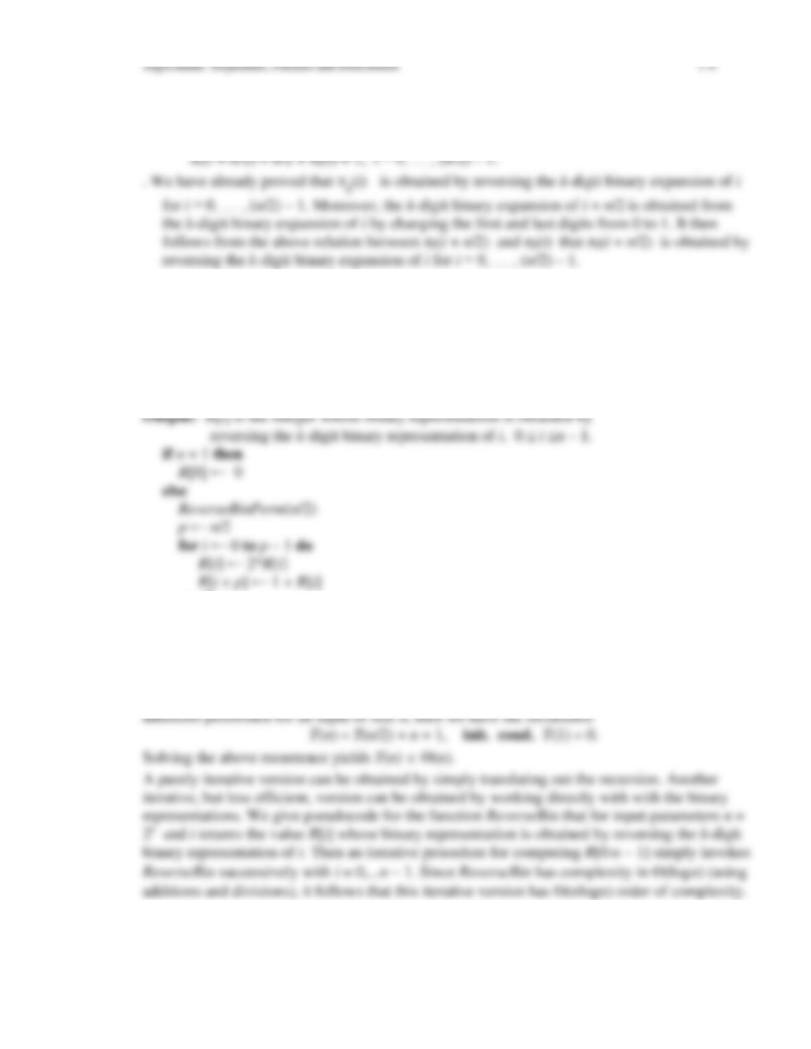
22.6 We give a recursive procedure that avoids binary representations altogether, and has linear
complexity.
procedure ReverseBinPerm(n) recursive
Input: n (a positive integer such that n = 2k )
R[0:n – 1] (a global array of size n)
endfor
endif
end ReverseBinPerm
We measure the complexity of ReverseBinPerm by using multiplications, divisions, and
additions as our basic operations. If T(n) denotes the total number of multiplications and
function ReverseBin(i,k)
Input: i (an integer such that 0 ≤ i ≤ 2k – 1
k (a positive integer)
Algorithms: Sequential, Parallel and Distributed 1-5
Output: the integer whose binary representation is obtained by reversing the k-digit binary
endwhile
//Compute the number represented (in reverse order) by Digits[0:k–1]
n ← n/2
Sum ← n
for j ← k-2 downto 0 do
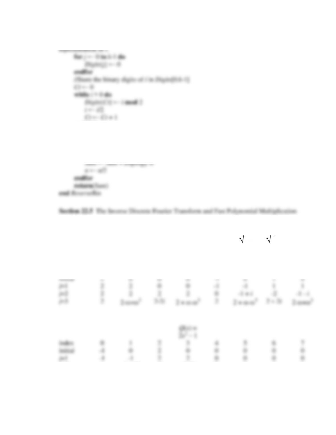
22.8 a) We show the state of the the matrix b[0:7] after each iteration of the outer loop,
for j ← 1 to k do, in the procedure FFT (see pp. 703-704). Here = i=(1+i)/ 2 .
P(x) =
x3–x+2
index
0
1
2
3
4
5
6
7
initial
2
0
0
0
-1
0
1
0
j=1
2
2
0
0
-1
-1
1
1
j=2
2
2
2
2
0
-1 + i
-2
-1 – i
j=3
2
2-+3
2-2i
2 + –3
2
2 + –3
2 + 2i
2-+3
Q(x) =
2x2 – 1
index
0
1
2
3
4
5
6
7
initial
-1
0
2
0
0
0
0
0
j=1
-1
-1
2
2
0
0
0
0
j=2
1
-1 + 2i
-3
-1 -2i
0
0
0
0
j=3
1
-1 + 2i
-3
-1 -2i
1
-1 + 2i
-3
-1 -2i
b) Using the results from part a), we form the point-wise products P(1)Q(1), P(ω)Q(ω), …,
P(ω7)Q(ω7), yielding the following coefficient array:
Algorithms: Sequential, Parallel and Distributed 1-6
Index
0
1
2
3
4
5
6
7
2
-2-+4i-33
-6+6i
-2-3-4i–3
2
–2++4i+33
-6-6i
-2+3-4i+3
We now compute FFT on the above coefficient array using the 8th root of unity ω–1 = ω3 (so
that we are evaluating the polynomial represented by the coefficient array at the points
1, –ω3, –i, –ω, -1, ω3, i, ω). We obtain:
index
0
1
2
3
4
5
6
7
initial
2
2
-6+6i
-6-6i
-2-+4i-33
–2++4i+33
-2-3-4i–3
-2+3-4i+3
j=1
4
0
–12
12i
-4+8i
-2-63
-4-8i
-6-23
j=2
-8
12
16
–12
-8
-4
16i
–123
j=3
–16
8
32
–24
0
16
0
0
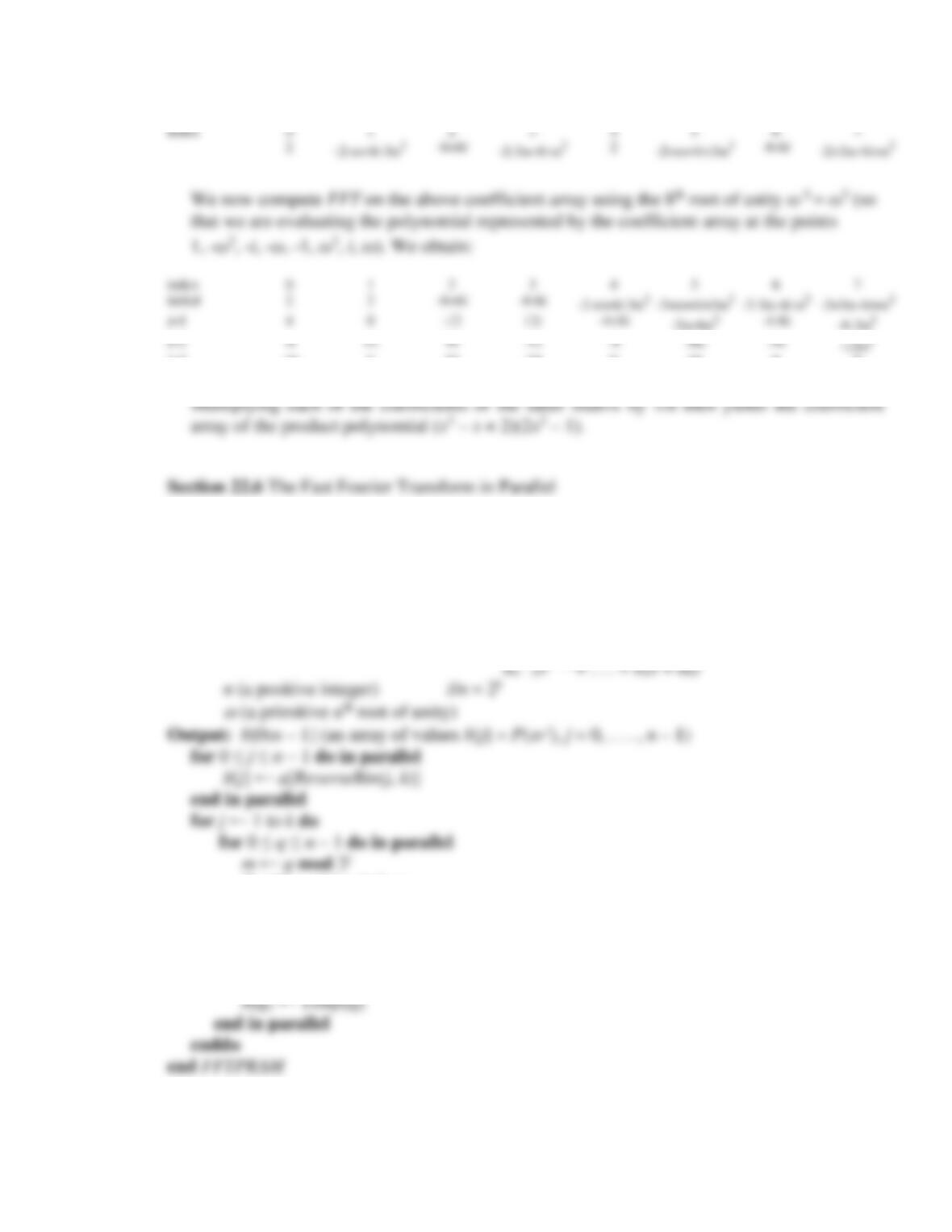
22.9 In the following pseudocode for FFTPRAM, the pseudocode for the iterative function
ReverseBin(i, k) is given in the solution to Exercise 22.6.
procedure FFTPRAM(a[0:n – 1], n,
, b[0:n – 1])
Model: EREW PRAM with n processors
Input: a[0:n – 1] (an array of coefficients of the polynomial P(x) =
if q/2j mod 2 = 0 then
Temp[q] ← b[q] + (
n/2j)m * b[q + 2j–1]
else
Temp[q] ← – (
n/2j)m * b[q] + b[q – 2j-1]
endif
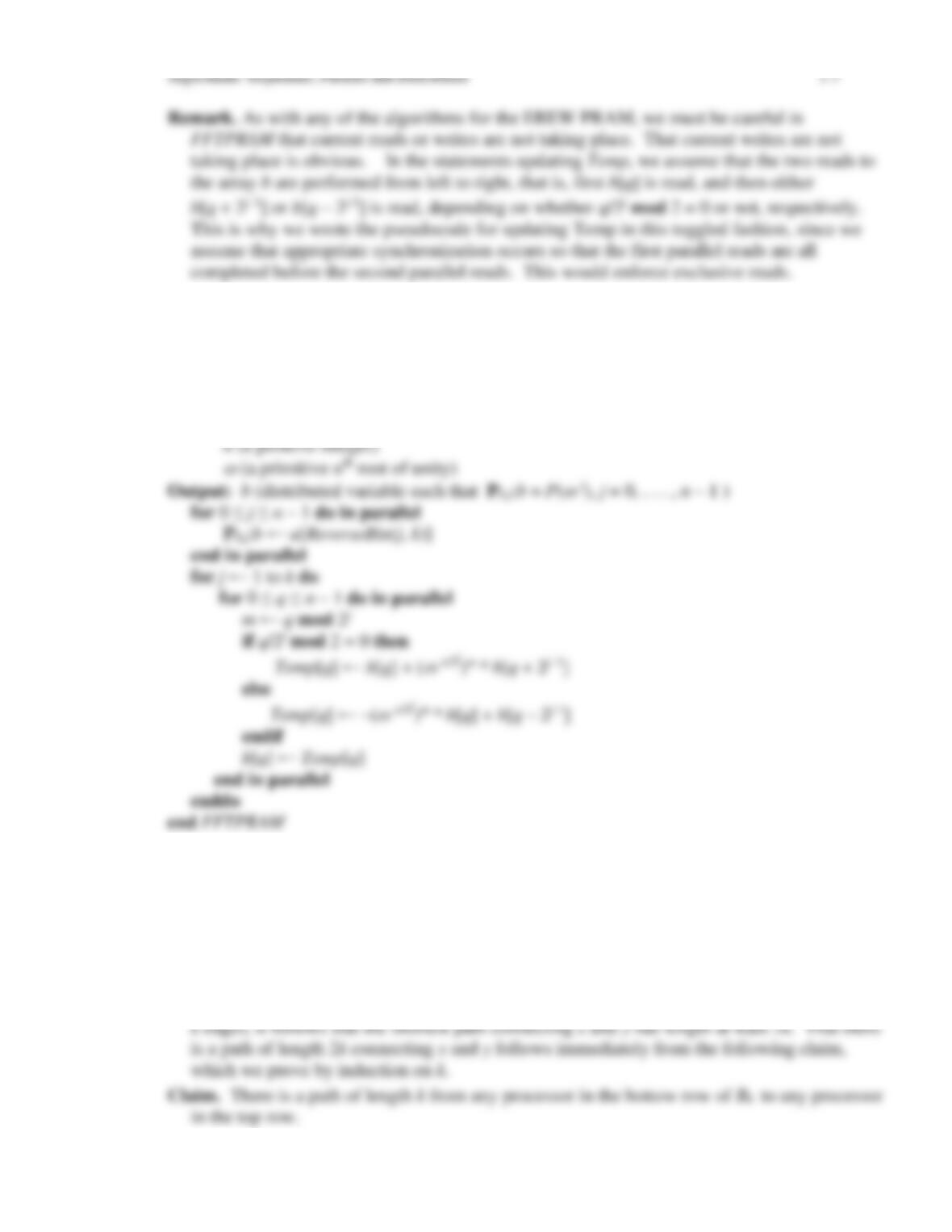
22.10
procedure FFTButterfly (a[0:n – 1], n,
, b)
Model: Butterfly Network Bk with n(log2n + 1) processors, n = 2k.
Input: a (an array of coefficients of the polynomial P(x) =
an – 1xn – 1 + . . . + a1x + a0 known to all processors P0,m)
22.11 It is clear that the maximum degree of the butterfly network Bk is 4 (see Figure 22.10). To
see that the diameter of Bk is 2k, note from Figure 22.10 that any path connecting a
processor x in the first half of the bottom row to a processor y in the second half of the
bottom row must go through a processor in the top row, and that the diameter of Bk is
achieved by the shortest of such paths. Since any path from the bottom level to the top uses
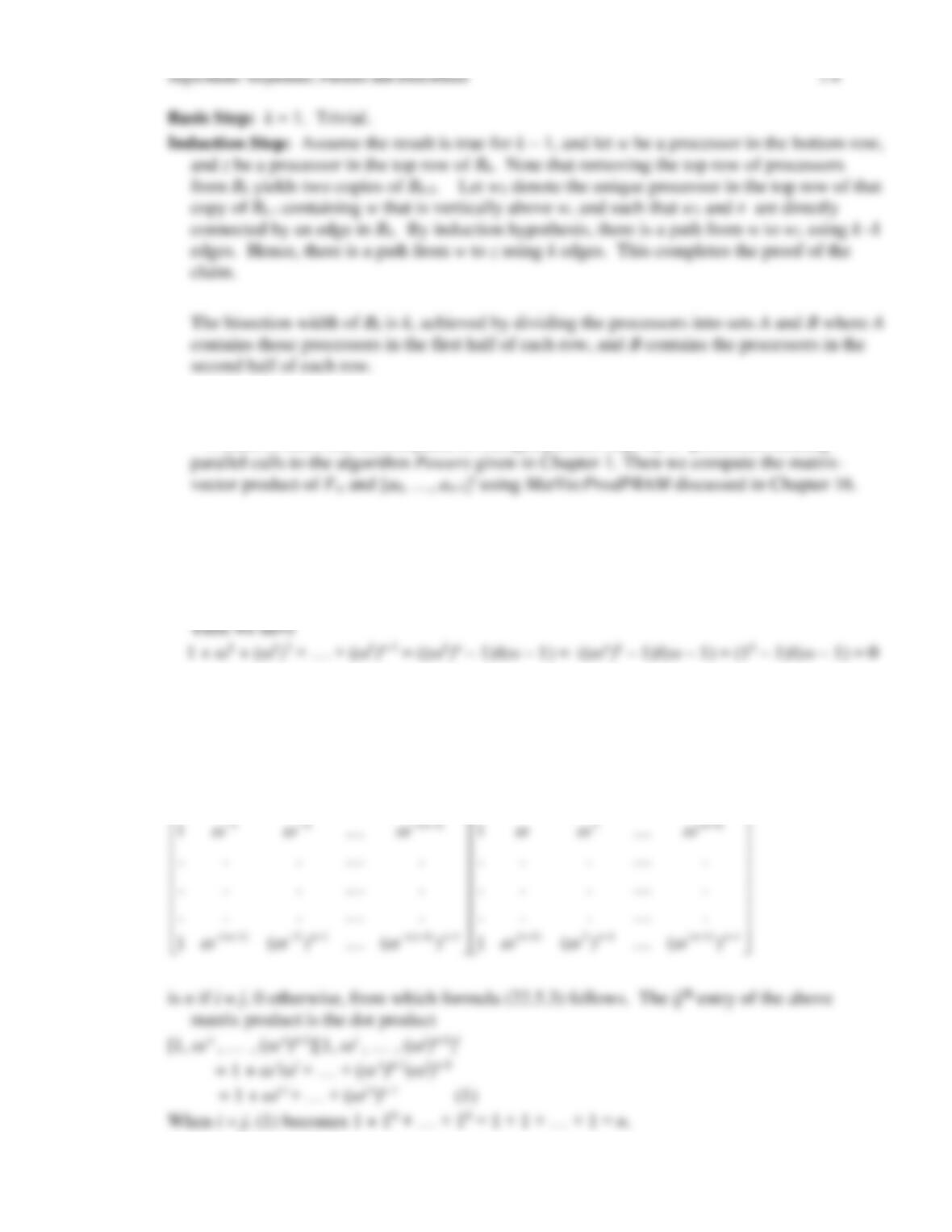
22.12 a) The matrix Fω given in (13.6.2) representing DFTω has ijth entry fij = ωij, i,j = 0, … , n
– 1. Each of these can be computed in (logn) parallel steps by n2 processors making
Additional Exercises
22.14 Let ω be a primitive nth root of unity, and suppose k is an integer such that 0 < k < n.
22.15 Note: This exercise was repeated in first printing of the book as Exercise 22.2. In
subsequent printings, this exercise is to prove Formula (22.5.3), whose proof we give here.
For 0 ≤ i,j, ≤ n – 1, we show that the ijth entry of the matrix product
−
−−−−
)1(2
)1(21
....
1
1111
....
1
1111
n
n
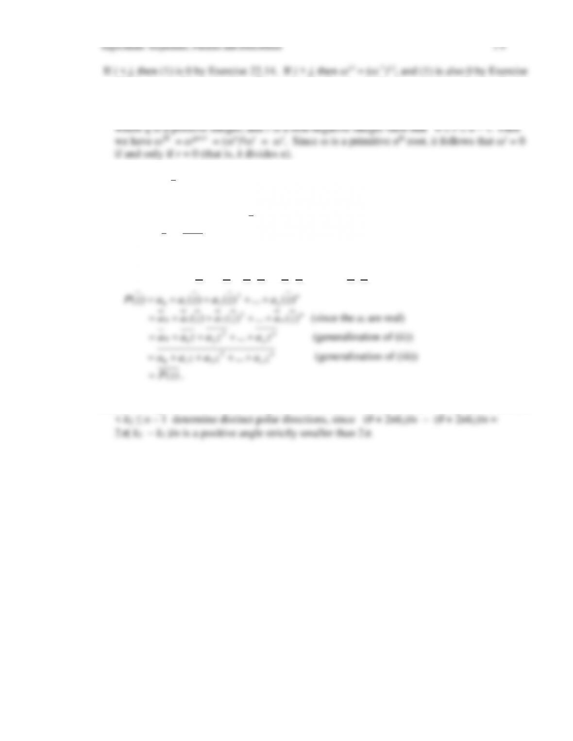
22.14, since ω-1 is a primitive nth root of unity if and only if ω is a primitive nth root of unity.
22.16 Let ω be a primitive nth root of unity. Suppose k is a positive integer such that k = qn+r,
22.17 a) z and
z
are symmetric about the x-axis.
c) Suppose P( z ) = a0 + a1( z ) + a2( z )2 + … + an( z )n where the coefficients ai are real, 0 i
n, and P(z) = 0. The result
0)( =zP
then follows from the formula
)()( zPzP =
.
To establish this formula, using the generalization of the formulas a) (ii) and (iii) of this
exercise to n complex numbers, we have
22.18 For a given value of
, two angles of the form (θ + 2πk1)/n and (θ + 2πk2)/n, where 0 ≤ k1