
Algorithms: Sequential, Parallel and Distributed 1-1
Chapter 15
Introduction to the Design of Parallel Algorithms
At a Glance
Table of Contents
• Overview
• Objectives
• Instructor Notes
• Solutions to Selected Exercises

Algorithms: Sequential, Parallel and Distributed 1-2
Lecture Notes
Overview
In Chapter 15 we introduce parallel algorithms and architectures. Shared memory (PRAMs)
and distributed memory (interconnection network) models are discussed and contrasted. SIMD
versus MIMD models, as well as EREW, CREW, and CRCW models are discussed and
illustrated. Some basic interconnection network models are introduced, such as meshes, trees,
and hypercubes, and goodness measures for these models are discussed. Communication
Chapter Objectives
After completing the chapter the student will know:
• The main approaches and architecture issues involved in the design and analysis of parallel
algorithms
• The difference between shared memory and distributed memory parallel machines
• The SIMD versus MIMD paradigm
• The various models of PRAMs, EREW, CREW, and CRCW, and how algorithms must take
these models into account
Algorithms: Sequential, Parallel and Distributed 1-3
Instructor Notes
Our pseudocode conventions for parallel algorithms is given in Appendix. G. Even though the
student might not have access to a parallel machine, it is important to expose the student to the
ideas of parallel programming, since these machines will undoubtedly become more common
and available as technology advances. Moreover, the ideas presented in this chapter are also
helpful in understanding distributed algorithms as discussed in Chapters 18 and 19. However,
it is true that distributed algorithms are perhaps more dominant today with the emergence of
cluster and grid computing, and such things as the ready availability of relatively inexpensive
Beowulf clusters. Also, distributed algorithms on Beowulf clusters using the MPI
programming library can be simulated on a single processor using freely available software
(see Chapter 18). In any case, while the material in Chapters 15 and 16 is helpful to the
understanding of the material in Chapters 18 and 19, the later material could be covered
without covering Chapters 15 and 16.
Solutions to Selected Exercises
Section 15.2 Architectural Constraints and the Design of Parallel Algorithms
15.1 a. In row-major ordering of Mq,q, the second coordinate (column coordinate) increases
the fastest. Hence, the natural way to generalize row-major to Mq,q,q is to have the coordinates
15.2 For any bipartition of the the vertices of Kn into equal size sets X and Y, the cut
15.3 Clearly the maximum distance between any two points of PTp is achieved by taking two
points at the deepest level, one in the left subtree of the root, and the other in the right subtree.
Algorithms: Sequential, Parallel and Distributed 1-4
15.4 a. The maximum degree of Mq,q,q is 6, achieved for any processor Pi,j,k where 0 < i,j,k < q
– 1, which is directly connected to processors Pi-1,j,k , Pi+1,j,k , Pi,j-1,k , Pi,j+1,k , Pi,j,k-1 , Pi,j,k+1
15.5 a. The maximum degree of
,qq
M
is 8, achieved for any processor Pi,j, where 0 < i,j < q –
1, which is directly connected to processors Pi-1,j , Pi+1,j , Pi,j-1 , Pi,j+1 , Pi-1, j-1 , Pi-1, j+1 , Pi-1, j-1 ,
,qq
M
15.6 a. Our search algorithm for Mq,q,q follows a similar strategy to that given in the text for
the two-dimensional mesh Mq,q. In the first stage, we broadcast the search element x to all
processors as follows. We broadcast x in q – 1 (sequential) steps to (the instantiation of the
distributed variable X for) processors Pi,j,k where j = 0 and k = 0. We then broadcast x in
q – 1 (parallel) steps to all processors where k = 0. Finally, in q – 1 (parallel) steps we
15.7 a. Assume that the numbers are stored in the distributed variable X. Similar to the gather
operation in the searching algorithm described in Exercise 15.6, q – 1 parallel addition steps we
can store the sum Pq-1,j,k:X + Pq-2,j,k:X + … + P0,j,k:X in P0,j,k:X. We then have reduced the
problem to summing q2 numbers on the two-dimensional mesh M0,q,q, which can be done in
*15.8 Consider Mq,q, where q =
p
. For convenience we will assume that q is even. Let X
denote the set of all processors Pi,j such that i ≤ (q/2) – 1 and let Y denote the remaining set of
processors. Then |X| = |Y| = p/2 and |C(X,Y)| = q. Thus, the bisection width of Mq,q belongs to
Ω(q). We now show that the bisection width belongs to O(q). The strategy is to “embed” the
complete graph Kp in Mq,q. The idea is to identify each processor of Mq,q with a processor of
15.9 Design the same as SumPRAM except that the last element in a list of size m is not paired
15.10 For k and m nonnegative integers, let bin(k,m) denote the k-digit binary representation of
the integer m (e.g., bin(4,2) = 0010). We denote the concatenation of two strings S and T by ST
(e.g., bin(4,2)0 = 00100 = bin(5,4) and bin(4,2)1 = 00101 = bin(5,5)). By convention, we
define bin(0,0) = ε.
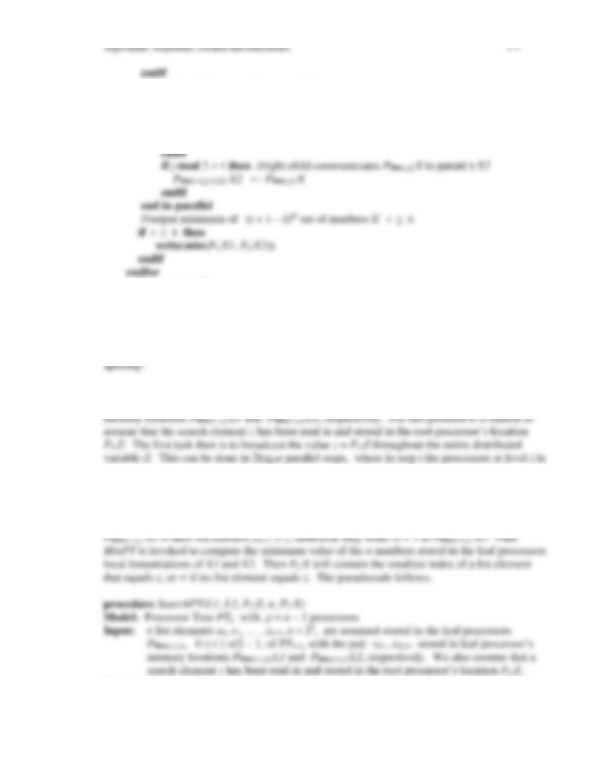
a. The following procedure finds the minimum of the n real numbers x0, x1, … , xn-1, n = 2k ,
Pbin(i-1,j/2):X1 ← Pbin(i,j):X
endif
if j mod 2 = 1 then //right child communicates Pbin(i,j):X to parent’s X2
Pbin(i-1,(j-1)/2):X2 ← Pbin(i,j):X
endif
Model: Processor Tree PTp with p = n – 1 processors
Input: There are m input steps, where at each input step n = 2k real numbers xj,0, xj,1, … , xj,n-1,
1 ≤ j ≤ m, are concurrently input in two steps into the leaf processors Pbin(k–1,i), 0 ≤ i ≤
n/2 – 1, with the pair xj,2i , xj,2i+1 read into leaf processor Pbin(k–1,i).
Output: There are m output steps, where at the jth output step, 1 ≤ j ≤ m, the minimum of the
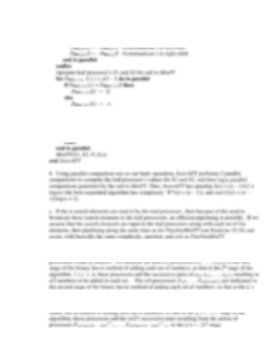
//compute minimums and communicate up
for Pbin(i,j), 1 ≤ i ≤ k – 1, 0 ≤ j ≤ 2i – 1 do in parallel
X ← min(X1,X2)
if j mod 2 = 0 then //left child communicates Pbin(i,j):X to parent’s X1
Pbin(i-1,j/2):X1 ← Pbin(i,j):X
end PipelineMinPT
d. Choosing parallel comparison as the basic operation, PipelineMinPT has complexity
W(n) = m + k – 1 = m + log2n – 1. Thus, PipelineMinPT has speedup
S(n) = (n – 1)/(1 + (log2n – 1)/m) and cost C(n) = (n – 1)(m + log2n – 1), which is order cost
optimal for O(m) ≥ O(logn). Note that for m >> log2n, we have essentially achieved linear
15.11 a. We assume that the list of n elements x0, x1, … , xn-1, n = 2k, reside in the leaf
processors Pbin(k–1,i), 0 ≤ i ≤ n/2 – 1, of PTn-1, with the pair x2i , x2i+1 stored in leaf processor’s
PTn-1 first communicate their local instantiation of Z to their left child’s local instantiation of X,
and then to their right child’s, i = 0, … , log2n – 1. In the next parallel step, leaf processors
Pbin(k–1,i) each compare their list element x2i to the search element z, writing ∞ to Pbin(k–1,i) :X1 if
their list element x2i ≠ z, otherwise they write 2i to Pbin(k–1,i) :X1. In the next parallel step, leaf
processors Pbin(k–1,i) each compare their list element x2i+1 to the search element z, writing ∞ to
Output: the smallest index i of an list element xi that equals the search element z resides in
Pε:X, or ∞ resides there if no list element equals z
Algorithms: Sequential, Parallel and Distributed 1-8
for i ← 0 to n/2 – 2 do //broadcast the search element Pε:Z throughout PTn-1
for Pbin(i,j), 0 ≤ j ≤ 2i – 1 do in parallel
endif
if Pbin(k-1,i):L2 = Pbin(k-1,i):Z then
Pbin(k-1,i):X2 ← 2i + 1
else
Pbin(k-1,i):X2 ← ∞
15.12 Suppose we have m sets of n numbers, xj,0, xj,1, … , xj,n–1, n = 2k, 1 ≤ j ≤ m. The
pipelining algorithm for computing the sums of each set of numbers on the PRAM with n – 1
1)st stage of the algorithm, these processors add the (n/4) successive pairs resulting from the
action of processors P0, … , P(n/2)-1 in the jth stage. In general, for a given i, 1 < i ≤ n/2i, the
n/2i processors P(n/2)+(n/4)+…+(n/2i-1 ), … , P(n/2)+(n/4)+…+(n/2i )-1 are dedicated to the ith stage of the
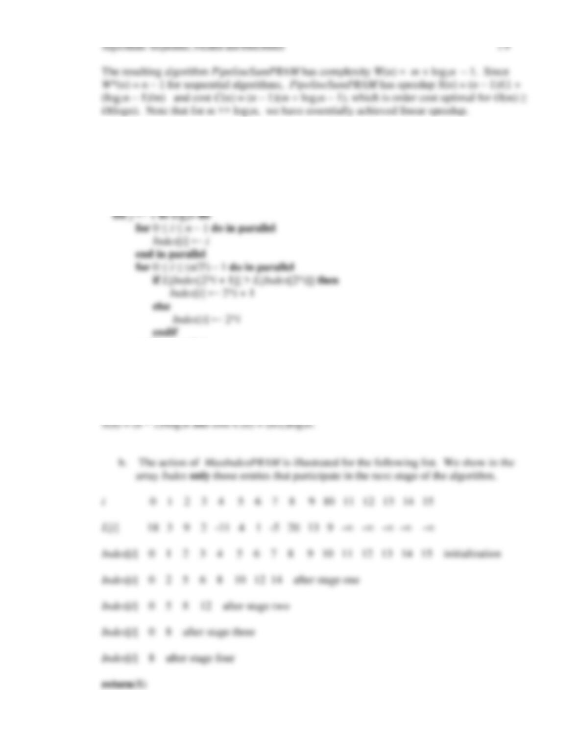
15.13 a.
function MaxIndexPRAM(L[0:n – 1])
Model: EREW PRAM with p = n/2 processors
Input: L[0:n – 1] (a list of size n, n = 2k)
Output: the (smallest) index of a list element of maximum value in L
end in parallel
endfor
return(Index[0])
end MaxIndexPRAM
MaxIndexPRAM performs log2n parallel comparison steps, so it has speedup
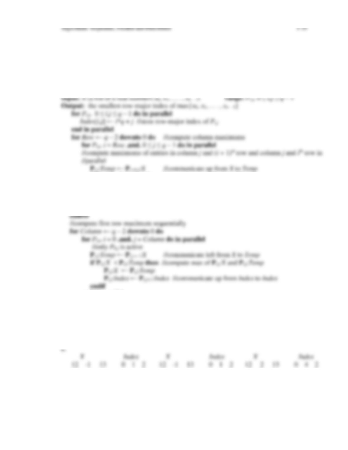
15.14 a. In our pseudocode for , we assume that since X is an input variable only, it is safe to
change its values without changing the corresponding distributed variable that is used in
the calling argument list.
function MaxIndex2DMesh(X,n)
Model: two-dimensional mesh Mq,q with p = n = q2 processors
if Pi,j:X < Pi,j:Temp then //compute max of Pi,j:X and Pi,j:Temp
Pi,j:X ← Pi,j:Temp
Pi,j:Index ← Pi +1,j:Index //communicate up from Index to Index
endif
end in parallel
end in parallel
endfor
return(P0,0:Index)
end MaxIndex2DMesh
MaxIndex2DMesh performs 2q – 2 parallel comparison steps.
-10 2 11 3 4 5 9 2 11 6 4 5 9 2 11 6 4 5
9 –∞ –∞ 6 7 8 9 –∞ –∞ 6 7 8 9 –∞ –∞ 6 7 8
Initial Stage After Stage one After Stage two
15.16 To remove concurrent reads and writes we allocate two two-dimensional arrays LL[0:n –
1 , 0:n – 1] and Win[0:n – 1,0:n – 1]. We assign LL[i, j] the value L[i] by broadcasting the
value L[i] to LL[i,0:n – 1] concurrently for each i, 0 i n – 1. This requires log2n steps.
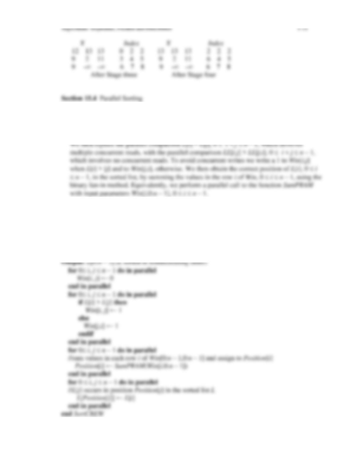
15.17 The following procedure sorts a list L[0:n – 1] of size n on the CREW PRAM in
logarithmic time using n2 processors.
procedure SortCREW(L[0:n – 1])
Model: CREW PRAM with p = n2 processors
Input: L[0:n – 1] (an array of n list elements in shared memory)