
Chapter 12
Minimum Spanning Tree and Shortest Path Algorithms
At a Glance
Table of Contents
• Overview
Lecture Notes
Overview
In this chapter we discuss two fundamental problems for (real) weighted graphs and
digraphs—the minimum spanning tree problem and the shortest path problem. We begin
by discussing Kruskal’s algorithm, which is based on the Greedy method, and involves
growing forests. We then discuss another classical minimum spanning tree algorithm,
Prim’s algorithm, which is also based on the greedy method, but involves growing a
spanning tree from a root vertex.
In the second part of this chapter we discuss three shortest path algorithms. We first
discuss the Bellman-Ford algorithm for computing shortest paths from a given root vertex
to other vertices, or determining the existence of a negative cycle. We then discuss
Dijkstra’s shortest path algorithm, which is based on a Greedy strategy similar to Prim’s.
Dijkstra’s algorithm is more efficient then the Bellman-Ford algorithm, but requires the
precondition that all edge weights are positive. Finally, we discuss Floyd’s algorithm for
computing all-pairs shortest paths, which is based on a dynamic programming strategy
that uses the principle of optimization.
Chapter Objectives
After completing the chapter the student will know:
• The design and analysis of Kruskals’ algorithm using the greedy method
• Efficient implementation of Kruskal’s algorithm using disjoint sets and union and
find algorithms
• The design and analysis of Prim’s algorithm using the greedy method
• The comparison of the computing times of Kruskal’s and Prim’s and for what
input graphs one would be more efficient than the other
• The ad hoc strategy used in the design of the Bellman-Ford algorithm and its
analysis
• The greedy strategy used in the design of Dijkstra’s algorithm and its analysis
Instructor Notes
It is worth pointing out in Kruskal’s algorithm that two forest implementations are
involved: the parent array forest implementation using the union and find algorithm for
maintaining the vertex sets of the current forest in order to test whether the next edge can
be added withouth creating a cycle, and the forest being created in the weighted graph
that will ultimately be the Kruskal minimum spanning tree. The vertex sets in both
forests are the same, but the student should bear in mind that the forest maintained by the
union and find algorithm is simply an efficient data structure for the disjoint set ADT as
discussed in Chapter 4.
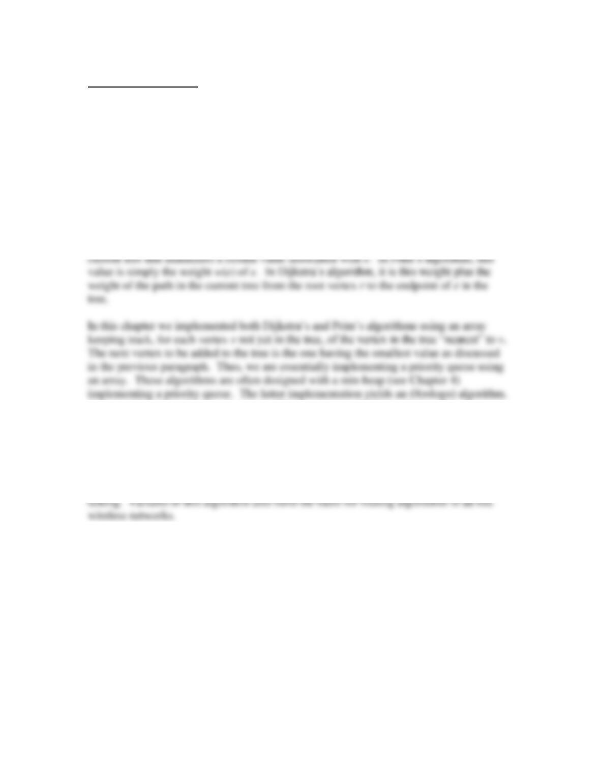
Dijkstra’s algorithm is similar to Prim’s in that we choose an edge e in the cut set of the
A more efficient implementation uses a Fibonacci heap, yielding a O(m + nlogn)
algorithm.
A generalization of Dijkstra’s algorithm, called A*-search, is a fundamental search
strategy in artificial intelligence applications (see Chapter 23).
In Chapter 19 we will adapt the Bellman-Ford algorithm to the distributed network
Solutions to Selected Exercises
Section 12.1 Minimum Spanning Tree
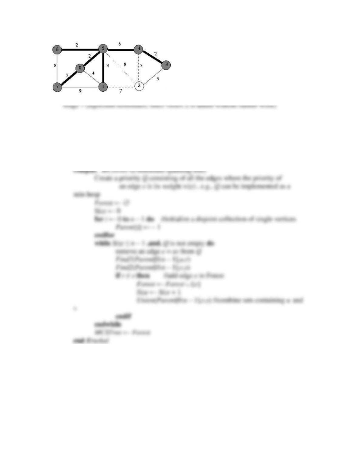
12.1 a) Procedure Kruskal chooses edges in increasing order of their costs, rejecting an
edge if it forms a cycle with the edges previously chosen. Thus, the action of Kruskal
is as follows, where on ties we choose an edge having the smallest vertex as an
endpoint.
{0,5}, {3,4}, {5,6}, {0,7}, {2,4}, {1,5}, {0,1} rejected because of cycle 015, {4,5}
Stage 1
i
0
1
2
3
4
5
6
7
0
4
5
6
Nearest[i]
4
0
7
∞
∞
3
∞
9
Parent[i]
1
-1
1
–
–
1
–
1
InTheTree[i]
F
T
F
F
F
F
F
F
i
0
1
2
3
4
5
6
7
Nearest[i]
2
0
7
∞
6
3
2
9
Parent[i]
5
-1
1
–
5
1
5
1
InTheTree[i]
F
T
F
F
F
T
F
F
Nearest[i]
2
0
7
∞
6
3
2
3
Parent[i]
5
-1
1
–
5
1
5
0
InTheTree[i]
T
T
F
F
F
T
F
F
0
4
5
6
2
3
4
5
6
7
2
3
7
2
3
7
i
0
1
2
3
4
5
6
7
Stage 3
Stage 5
i
0
1
2
3
4
5
6
7
Nearest[i]
2
0
3
2
6
3
2
3
Parent[i]
5
-1
4
4
5
1
5
0
InTheTree[i]
T
T
F
F
T
T
T
T
i
0
1
2
3
4
5
6
7
2
3
7
4
5
6
i
0
1
2
3
4
5
6
7
Nearest[i]
2
0
7
∞
6
3
2
3
Parent[i]
5
-1
1
–
5
1
5
0
InTheTree[i]
T
T
F
F
F
T
T
F
Nearest[i]
2
0
7
∞
6
3
2
3
Parent[i]
5
-1
1
–
5
1
5
0
InTheTree[i]
T
T
F
F
F
T
T
T
Nearest[i]
2
0
3
2
6
3
2
3
Parent[i]
5
0
4
4
5
1
5
0
InTheTree[i]
T
T
F
T
T
T
T
T
2
3
7
2
3
7
4
5
6
2
3
7
i
0
1
2
3
4
5
6
7
4
5
6
12.2 Pseudocode for implementation of Kruskal’s algorithm where
procedure Kruskal(G,w,MCSTree)
Input: G (a connected graph with vertex set V of cardinality n
and edge set E = {ei = uivi | i {1,…,m}})
w (a weight function on E)
12.3 a) Clearly, adding an edge e to a tree T creates a cycle since a tree is a minimal
connected graph without cycles. Assume that the resulting graph H has two or more
cycles, say C1 and C2. Clearly, both these cycles contain edge e. Now consider the
subgraph C induced by the symmetric difference of C1 and C2, that is, C is the
subgraph consisting of all the edges that lie in one of C1 and C2, but not both. It is
12.5 Construct a new graph G’ from G by adding, for each pair of non-adjacent vertices i
and j, an edge joining i and j having weight
(where
represents a sufficiently
12.6 The proof that Prim’s algorithm yields a minimum cost spanning tree is similar to
the proof of the correctness of Kruskal’s algorithm. Let P be the spanning tree
generated by Prim’s algorithm, and suppose that the edges of P are generated in the
sequence e1,e2,…,en-1 . Suppose to the contrary that P is not a minimum cost tree.
12.7 The worst-case occur when G is a complete graph. When the ith cut is computed at
stage i there are i nodes in the tree and n – i nodes not in the tree. Thus, each node of the
tree is adjacent to n – i nodes not in the tree, so that the cut has size i(n – i). We will need
12.8 We implement Prim’s algorithm using a priority queue whose operations include
the operation of changing the priority value of an element as well as the usual operations
of enqueue and dequeue
procedure Prim2(G,w,Parent[0:n – 1])
Input: G (a connected graph with vertex set V and edge set E)
for Stage ← 1 to n – 1 do
dequeue vertex u //u has the highest priority value, i.e., the smallest value, of all
//the elements in Q
InTheTree[u] ← .true. // add u to T
for each vertex v such that uv E do // update priority value of v and Parent[v]
12.9 Consider the digraph with vertex set V = {0,1,2} and edge set E = {(1,0),(2,0),
(1,2)}, where (1,2) has weight 1, (1,0) has weight 2 and (2,0) has weight 3. The
12.10 a)
Index
1
1
scan 0:
Dist:
0
Parent:
-1
scan 1:
Dist:
0
0
0
1
4
8
7
2
5
Parent:
8
-1
3
1
5
3
7
1
5
scan 2:
Dist:
0
0
0
1
4
8
1
-4
5
Parent:
8
-1
3
1
5
3
7
0
5
scan 3:
Dist:
0
0
0
1
4
8
1
-4
5
Parent:
8
-1
3
1
5
3
7
0
5
scan 4:
Dist:
0
0
0
1
4
8
1
-4
5
Parent:
8
-1
3
1
5
3
7
0
5
scan 5:
Dist:
0
0
0
1
4
8
1
-4
5
Parent:
8
-1
3
1
5
3
7
0
5
scan 6:
Dist:
0
0
0
1
4
8
1
-4
5
Parent:
8
-1
3
1
5
3
7
0
5
scan 7:
Dist:
0
0
0
1
4
8
1
-4
5
Parent:
8
-1
3
1
5
3
7
0
5
scan 8:
Dist:
0
0
0
1
4
8
1
-4
5
Parent:
8
-1
3
1
5
3
7
0
5
b)
Index
1
1
scan 0:
Dist:
0
Parent:
-1
scan 1:
Dist
3
2
0
Parent:
6
7
-1
scan 2:
Dist
1
3
1
2
5
9
0
5
6
Parent:
8
6
3
7
5
3
-1
2
5
scan 3:
Dist
1
-1
1
2
5
9
0
-3
5
Parent:
8
2
3
1
5
3
-1
1
5
scan 4:
Dist
-1
-1
-1
0
3
7
0
-3
4
Parent:
8
2
3
1
5
3
-1
1
5
scan 5:
Dist
-1
-3
-1
0
3
7
0
-5
4
Parent:
8
2
3
1
5
3
-1
1
5
scan 6:
Dist
-3
-3
-3
-2
1
5
0
-5
2
Parent:
8
2
3
1
5
3
-1
1
5
scan 7:
Dist
-3
-5
-3
-2
1
5
-2
-7
2
Parent:
8
2
3
1
5
3
7
1
5
scan 8:
Dist
-5
-5
-5
-4
-1
3
-2
-7
0
Parent:
8
2
3
1
5
3
7
1
5
A negative cycle exists, as detected by the fact, for example, that
dist(1) = -5 > dist(2) + c(21) = -5 -2 = -7.
12.11 a) Replace the statement
for Pass ← 1 to n do
with the statements
i ← 1
flag ← 1
Best-case complexity. Consider any input weighted input digraph (D,w) that has no
negative cycles. Then the following ordering of the edges results in the improved
version of BellmanFord given in part a) performing exactly two edge scans, i.e., the
for loop is executed only two times. Let T be any shortest path tree. Order the edges
such that all the edges not in the tree occur after any edges in the tree, and edges in the
12.12 Replace the statement
for each edge uv
E
with the statements
12.13 Suppose to the contrary that a weighted digraph D contains a shortest path having
more than n – 1 edges, i.e., P = u0 e1 u1 e2 u2 …, ek uk, where k ≥ n edges. Since P
12.14 Using an analogous argument to that given in the proof of Lemma 12.2.1 on page
380, Lemma 12.2.1 can be extended to hold for the nth iteration, even if negative
cycles are present if shortest path is replaced with shortest walk, where a walk is the
same as a path except repeated vertices and edges are allowed. First suppose there is
no negative cycle, and consider a shortest walk W of length n from the root r to a