Algorithms: Sequential, Parallel and Distributed 1-1
Chapter 11
Graphs and Digraphs
At a Glance
Table of Contents
• Overview
• Objectives
• Instructor Notes
• Solutions to Selected Exercises
Algorithms: Sequential, Parallel and Distributed 1-2
Lecture Notes
Overview
In Chapter 11 we give a brief introduction to the theory of graphs, including the definition of
some basic graph concepts such as paths, degree, isomorphism, coloring, planarity, and so
forth. This is followed by a discussion of the standard implementations of the graph and
digraph ADTs. We also discuss the two classical searching algorithms depth-first search and
bread-first search and the associated traversal algorithms depth-first traversal and breadth-first
traversal. We finish the chapter by showing how the reverse explored numbering solves the
problem of efficiently determining a topological sorting of the vertices in a directed graph
without cycles (dag).
Chapter Objectives
After completing the chapter the student will know:
• The importance of graphs and digraphs in modeling problems and networks
• The basic definitions relating to graphs and digraphs
• The two main methods of implementing graphs and digraphs, namely, adjacency matrices
versus adjacency lists, and the advantages of each implementation
• The importance of topological sorting in digraphs, and how the reverse explored numbering
solves this problem efficiently
Instructor Notes
The concept of a digraph is a generalization of a graph in the sense that any given graph G can
be thought of as beings combinatorially equivalent to the symmetric digraph obtained by
replacing each edge {u,v} with the two directed edges (u,v) and (v,u). Hence, algorithms
designed for digraphs can typically be applied to graphs.
Algorithms: Sequential, Parallel and Distributed 1-3
Solutions to Selected Exercises
Section 11.1 Graphs and Digraphs
11.1 Note that each (directed) edge has exactly one tail and
)(vdout
counts the number of edges
having tail v. Thus, if we sum
)(vdout
over all the vertices vV, then each edge is counted
=
Vv out mvd )(
=
Vv in mvd )(
11.2 A tree is defined as a connected graph without cycles. We will show that a tree T contains
a unique path joining every pair of vertices u and v. Since T is connected there is at least one
11.3 We first show by induction that the number m of edges of any tree T is one less then the
number n of vertices of T, that is m=n-1. Clearly, the result is true for n=1 since the tree with
one node has no edges, establishing the basis step. Now assume the result is true for all trees
having n-1 vertices, and consider any tree T having n vertices. Let u be any leaf of T (that is,
11.4 Successively visit the vertices of G, coloring each vertex with any color different from its
11.5 In this exercise, we are assuming that the algorithms terminate once the first solution is
found.
a). The 3-coloring generated by backtracking is: 0,0,1, 2,1,2.
11.6
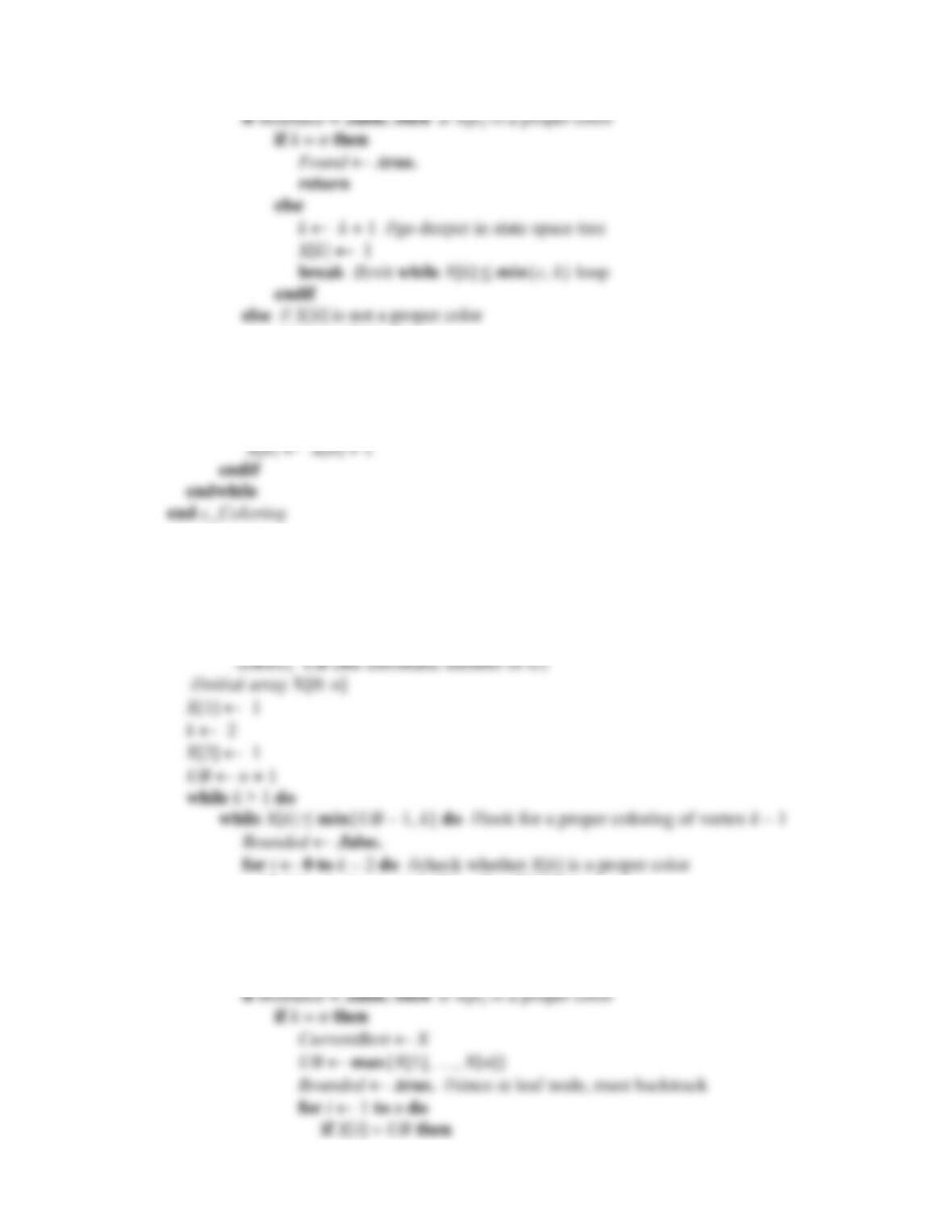
procedure c_Coloring (A[0:n – 1, 0:n – 1], X[0: n], c, Found)
Input: A[0:n – 1, 0:n – 1] (adjacency matrix of a graph G)
c (a positive integer)
Output: if Found = .true. then X[1], …, X[n] is a proper c-coloring of G, otherwise no
Bounded .true.
break //exit for loop
endif
endfor
Algorithms: Sequential, Parallel and Distributed 1-5
X[k] X[k] + 1
endif
endwhile
if Bounded = .true. then //vertex k – 1 cannot be properly colored: backtrack
k k – 1
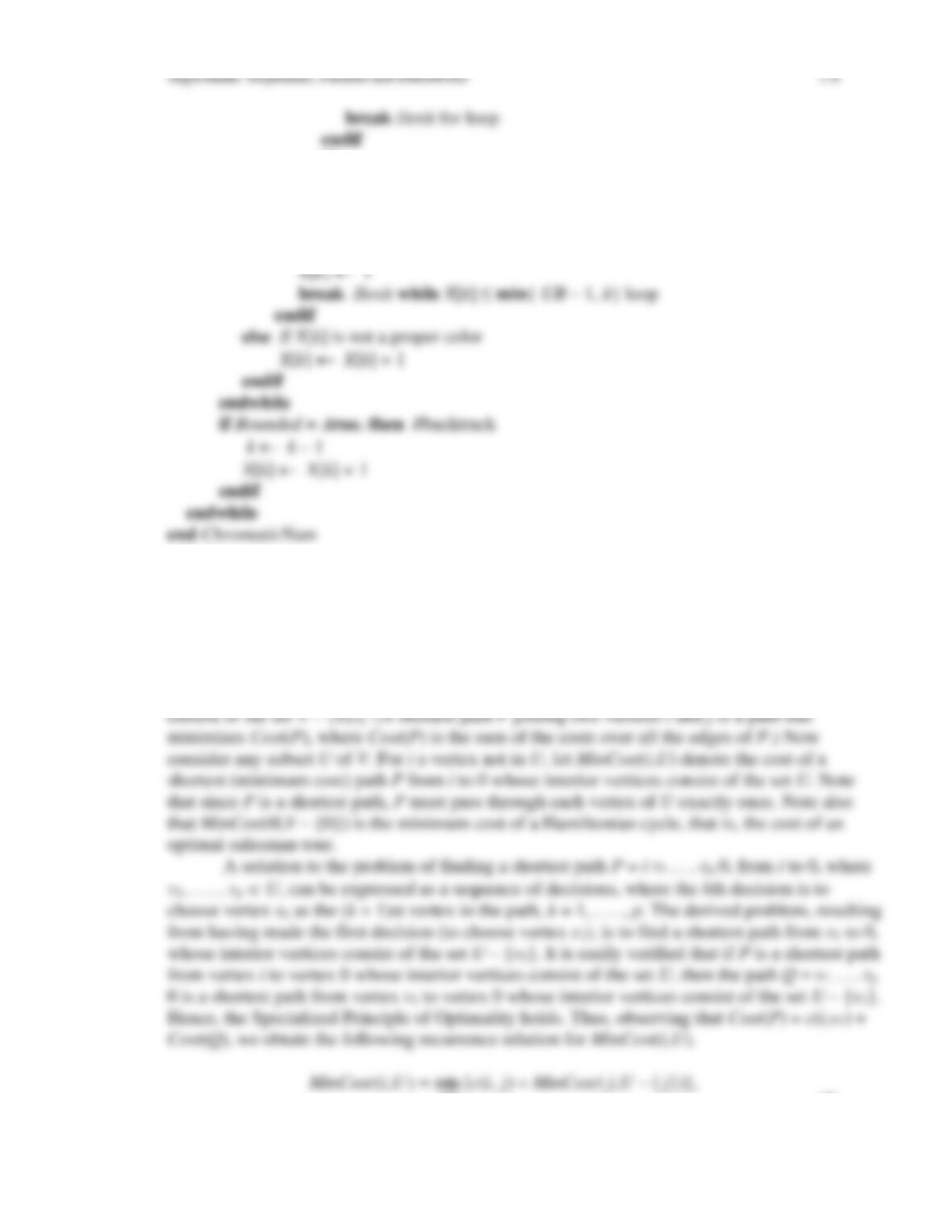
11.7
procedure ChromaticNum(A[0:n – 1, 0:n – 1], CurrentBest[0: n], UB)
Input: A[0:n – 1, 0:n – 1] (adjacency matrix of a graph G)
Output: CurrentBest[0: n] (an array where CurrentBest[1], …, CurrentBest[n] is a
proper coloring of the vertices 0, …, n – 1 using the minimum number of
if A[k – 1, i] = 1 .and. X[i + 1] = X[k] then
Bounded .true.
break //exit for loop
endif
endfor
endfor
k i
break //exit X[k] ≤ min{UB – 1, k}
else
k k + 1 //go deeper in state space tree
11.9 Consider a Hamiltonian cycle H of
ˆ
K
n
, where without loss of generality we assume that
vertex 0 is the initial and terminal vertex of H. Let i denote the first vertex visited by H after
leaving vertex 0, and let Hi denote the subpath of H from vertex i to vertex 0, which passes
through each vertex of
ˆ
K
n
once (such a path is called a Hamiltonian path). If H is a minimum
cost Hamiltonian cycle, then Hi must be a shortest path from i to 0 whose interior vertices
11),0,(),(
})},{,(),({min),(
−=
−+=
niiciMinCost
jUjMinCostjicUiMinCost Uj
cond. init.
(1)
Algorithms: Sequential, Parallel and Distributed 1-7
Recurrence relation (1) yields an algorithm for solving the Traveling Salesman problem.
Using Formula (1), we compute the values of MinCost(i,U) for all pairs i,U, where |U| = 1. We
then use Formula (1) to compute the values of MinCost(i,U) for all pairs i, U, where |U| = 2. In
(However, it is the cost of maintaining MinCost that contributes the major portion of the work
done by the algorithm.)
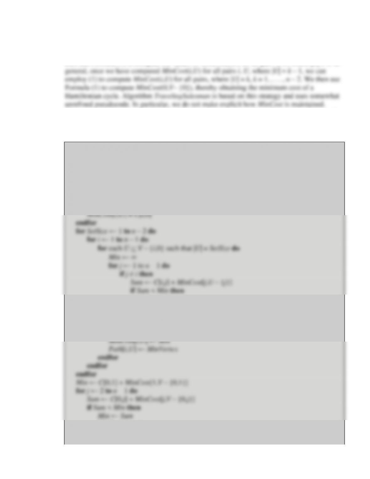
b) The following pseudocode is based on Formula (1).
procedure Traveling Salesman(C[0:n – 1,0: n – 1],Tour[0: n – 1],Cost)
Input: C[0: n – 1,0: n – 1] (cost matrix)
Output: Tour[0: n – 1] (Tour[i] is the ith vertex of a minimum cost Hamiltonian cycle, i = 0,
. . . , n – 1)
Cost (minimum cost of a Hamiltonian cycle)
for i ← 1 to n – 1 do
Min ← Sum
MinVertex ← j
endif
endif
endfor
MinVertex ← j
endif
endfor
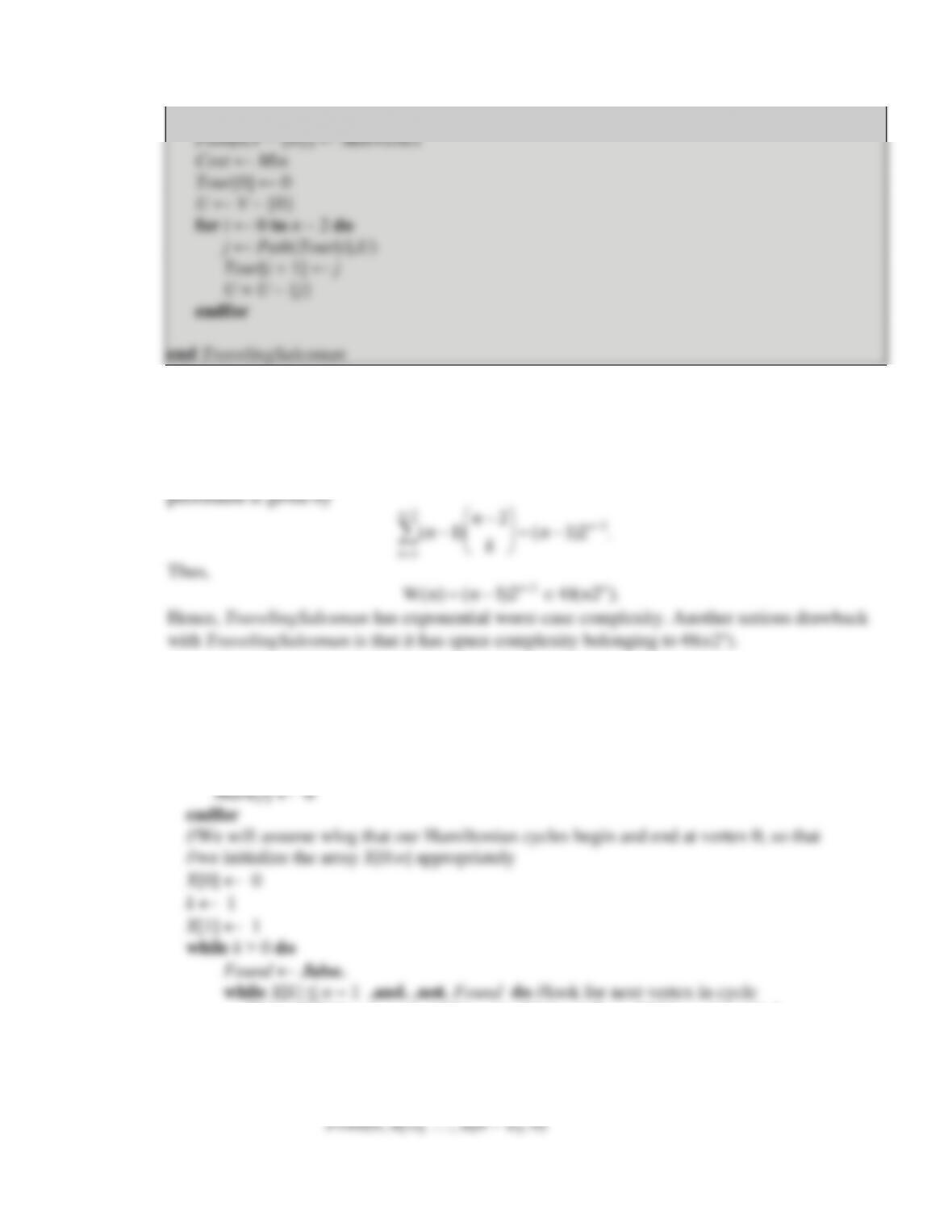
Algorithms: Sequential, Parallel and Distributed 1-8
{MinCost[0,V – {0}] = Min}
c) We now analyze the worst-case complexity W(n) of TravelingSalesman. We choose as our
basic operation an assignment to MinCost. For SetSize = k and i fixed, the number of sets U
V – {1,i} of size k is
n−2
k
. Thus, the total number of assignments to MinCost[i,U] that are
Hence, TravelingSalesman has exponential worst-case complexity. Another serious drawback
with TravelingSalesman is that it has space complexity belonging to (n2n).
11.10
procedure HamiltonianCycles(A[0:n – 1, 0:n – 1])
Input: A[0:n – 1, 0:n – 1] (adjacency matrix of a directed graph D)
Output: all Hamiltonian cycles of D are printed.
. for i 0 to n – 1 do
if Mark[X[k]] = 0 .and. A[X[k – 1 ], X[k]] = 1 then //X[k] can be added
Mark[X[k]] 1
Found .true.
if k = n – 1 then
if A[X[k], 0] = 1 then //Hamiltonian cycle found
X[k] 1
endif
else
X[k] X[k] + 1
endif
11.11
procedure TSP(A[0:n – 1, 0:n – 1], CurrentBest[0:n], UB)
Input: A[0:n – 1, 0:n – 1] (adjacency matrix of a weighted complete directed graph D)
Output: CurrentBest[0:n], (an optimal Hamiltonian cycle), UB (the cost of CurrentBest)
for i 0 to n – 1 do
Bounded .false.
while X[k] ≤ n – 1 .and. .not. Bounded do //look for next vertex in cycle
if Mark[X[k]] = 0 .and. PathCost + A[X[k – 1 ], X[k]] < UB then
if k = n – 1 then
temp PathCost + A[X[k – 1 ], X[k]] + A[X[k], 0]
X[k] 1
break //exit the while X[k] ≤ n – 1 .and. .not. Bounded loop
endif
else
X[k] X[k] + 1
11.13
procedure IndependentSet(A[0:n – 1, 0:n – 1], CurrentBest, LB)
Input: A[0:n – 1, 0:n – 1] (adjacency matrix of a graph G)
Output: CurrentBest (a largest independent set of vertices of G)
LB (the number of vertices in CurrentBest)
X[k] X[k – 1] + 1 //visit first child of E-node
else
X[k] X[k] + 1 //visit next child of E-node
endif
if X[k] > n – 1 then //no more children of E-node
if .not. Bounded then
if k > LB then
CurrentBest (X[1], … , X[k])
LB k
break //exit while ChildSearch
11.14 In the solution to this exercise and the next, as well as in the supplemental material, we
will exploit the following nice recursive structure of the hypercube Hk of dimension k. Recall
that Hk has vertices consisting of all 0/1 k-tuples, that is,
V(H)={(x1,x2,…,xk)|xi{0,1},i=1,…k} . Let V0 and V1
11.15 a) We prove that Hk is k-regular using induction. H0 is 0-regular, establishing the base
case. Now assume that Hk-1 is (k-1)-regular. Hk is recursively constructed from two copies
of Hk-1 by pairing corresponding vertices and joining each pair with edge. Thus, the degree
Algorithms: Sequential, Parallel and Distributed 1-12
11.16 We established in part (a) of Exercise 8.5 that Hk is k-regular. Thus, it follows from
11.17 The vertex set V of Hk consists of all 0/1 k-tuples x=(x1,x2,,xk) . It is easily seen
that we obtain a sub-hypercube of dimension j as the induced subgraph of a subset U of V if,
11.18 a) A cycle of size 15 (or 16) is 2-regular and has diameter 8.
b) The following 3-regular graph has diameter 5.
11.20 No. Assume to the contrary that such a graph G did exist. Then by Corollary 8.1.2,
5n=2m=88. But this implies that 88 is divisible by 54, a contradiction.
11.21 Let T be a 2-tree with I interior nodes and L leaf nodes. Note that every interior node has
degree 3 except the root node which has degree 2 and every leaf node has degree 1. Thus, by
Proposition 8.1.1
11.22 We assume that we are summing n numbers, where the n numbers are distributed
amongst the n=2k processors of Hk, and that the sum of the numbers is to be stored in
11.23 Clearly, if G has an Eulerian path from a to b, that is a path from a to b that contains
every edge of G then G is connected and every vertex has even degree but a and b.
Conversely, suppose G is connected, a and b have odd degree and every other vertex has
11.24 a) Procedures for adding and deleting an edge when G is implemented using its
adjacency matrix A[0:n – 1,0:n – 1]:
procedure AddEdge(A[0:n – 1,0:n – 1],i,j)
Input: A[0:n – 1,0:n – 1] (adjacency matrix of graph G=(V,E))
i,j (two vertices from V={1,2,…,n})
assume that the nodes of the adjacency lists are represented by a dynamic variable having
the following structure.
Algorithms: Sequential, Parallel and Distributed 1-14
Node = record
Info: InfoType
while Current null do .and. .not. Found do
if Current → Info = j then
Found ← .true.
else
Current ← Current →Next
Header[j] → Next ← New
endif
end AddEdge
The procedure for deleting a node involves searching the adjacency list pointed to by
Header[i] and deleting the node whose information field Info equals j, and then searching
11.25 When deleting an edge {i,j} we need only compute Headeri. Once we have found the
node corresponding to {i,j} in the adjacency list of node i, we can use the pointer p to go
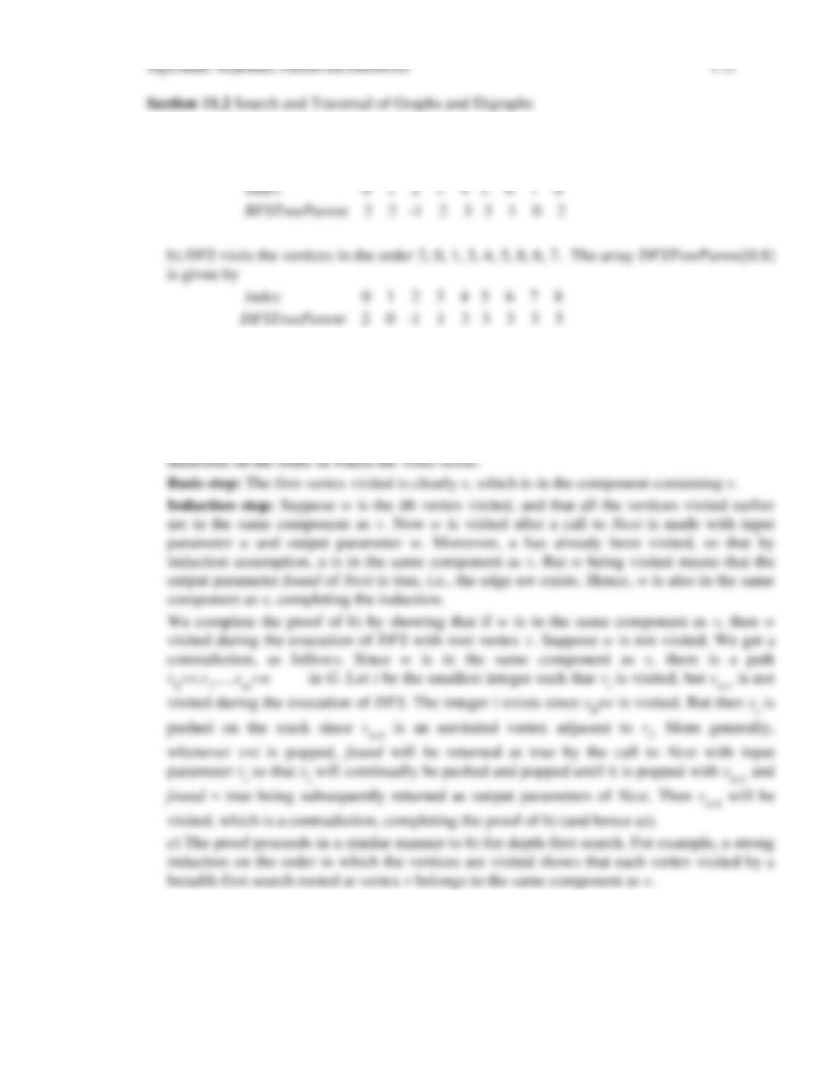
11.26 a) BFS visits the vertices in the order 2, 0, 1, 3, 8, 7, 6, 4, 5. The array
BFSTreeParent[0:8] is given by
11.27 Part a) follows from part b), with the understanding that a depth-search with root vertex v
visits precisely those vertices in the component of G containing v. Thus, we prove b) with
this understanding.
b) We use the nonrecursive version of DFS. We first show that every vertex visited during
the execution of DFS with root vertex v is in the same component as v. We use (strong)
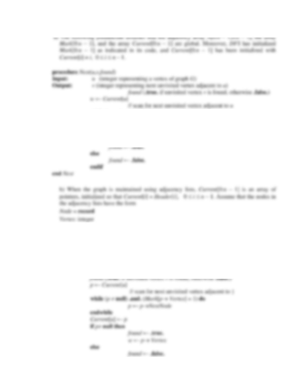
11.28 The pseudocode we need to give here for DFS is basically the same as given in the text
(recursive version on page 343 and iterative version on page 345-346). The only extra detail
we need to include is the pseudocode for finding the next unvisited node v in the
neighborhood of u, i.e., psuedocode for the procedure Next(u,v,found).
Algorithms: Sequential, Parallel and Distributed 1-16
while (w n) .and. (Mark[w] = 1 .or. A[u,w] = 0) do
w ← w + 1
endwhile
Current[u] ← w
if w n then
NextNode: → Node
end
Then the pseudocode for Next becomes
procedure Next(u,v,found)
Input: u (integer representing a vertex of graph G)
Output: v (integer representing next unvisited vertex adjacent to u)
11.29 The pseudocode we need to give here for BFS is basically the same as given in the text
11.30 In constructing the BFS-tree T rooted at vertex v node w is added to the tree as the parent
of u when w is first enqueued (in the for loop after dequeueing u in the pseudocode on page
348). An easy induction argument proves the following lemma.
Lemma. All nodes of distance strictly less than k from v are enqueued before any node of
distance k from v is enqueued.
11.31 We may assume without loss of generality that the DFS-forest is a tree (if not, we can
11.32 If there is a back edge then the path in the DFS-forest from u to v together with the
edges vu forms a directed cycle so that D is not a dag. Conversely, suppose there are no
11.33 a. Based on the previous exercise, compute a DFS-forest by calling DFTForest. If there
are no back edges then D is a dag, otherwise it is not. To make our algorithm slightly more
11.34 Perform a breadth-first traversal of the graph G = (V,E) keeping track of the parity of the
distance d(v) from v to the root vertex of the depth-first search tree containing v. It is easily
11.35 For each vertex vV, we find a smallest cycle Cv containing v, and then choose the
smallest cycle amongst these cycles. To find the smallest cycle through a given vertex v, we
11.36 We get the following array for TopList
TopList
0
1
2
3
4
5
6
7
8
9
10
11
12
13
14
7
9
8
5
14
13
12
6
4
2
3
1
10
11
0