Algorithms: Sequential, Parallel and Distributed, Second Edition 10-1
Chapter 10
Backtracking and Branch-and-Bound
At a Glance
Table of Contents
• Overview
• Objectives
• Instructor Notes
• Solutions to Selected Exercises

Algorithms: Sequential, Parallel and Distributed, Second Edition 10-2
Lecture Notes
Overview
In this chapter we discuss the backtracking and branch-and-bound paradigms, which are based
on searching a state space tree with an appropriate bounding function. We begin by defining
the concept of a state-space tree and give examples of variable and fixed-tuple state space trees.
We then describe (recursive and iterative versions of) the general backtracking strategy, which
we apply to solve the sum of subsets problem and the problem of finding tie board’s in the d×d
game of tic-tac-toe. This is followed by a discussion of the backtracking paradigm involving
both a static and dynamic bounding function for solving optimization problems. We finish the
chapter by discussing the general branch-and-bound strategy, which involves explicitly
maintaining the state space tree. In particular we discuss and compare the LIFO and FIFO
branch-and-bound searches of the state-space tree.
Chapter Objectives
After completing the chapter the student will know:
• The concept of a state space tree (variable and fixed-tuple) associated with a problem
• The general backtracking strategy (recursive and iterative version)
• The branch-and-bound strategy requires that portion of the state space tree currently
generated to be implemented explicitly, whereas in backtracking only the current path
needs to be maintained
Instructor Notes
Instructor should emphasize that in branch-and-bound that portion of the state space tree

of T in the same order regardless of the input to the algorithm. On the other hand, least
cost branch-and-bound discussed in Chapter 23 of Part V uses a least-cost heuristic to choose
the next node to expand. Searching state space trees can be generalized to searching state
space digraphs. In Chapter 23 of Part V we discuss the fundamental AI search strategy called
A* search, which is based on searching state space digraphs using a suitable heuristic to bound
the search.
Backtracking is particularly suitable for distributed computation, where different processors are
responsible for different portions of the state space tree. An implementation of backtracking in
a distributed setting is discussed in Chapter 18 of Part IV.
The recursive versions of backtracking are usually very elegant and simple in code. However,
since backtracking with clever heuristics is currently one of the only ways we know how to
solve NP-complete problems such as SAT, when applying backtracking to such problems it is
particularly important to write the code non-recursively for reasons of efficiency. Nevertheless,
the recursive versions of backtracking are often useful in formulating the non-recursive
versions. .
Solutions to Selected Exercises
Section 10.1 State-Space Trees
10.1 a. We are assuming the variable-tuple state-space tree in this exercise. Note that Pk and
Dk(x1, …,xk-1) are the same as for the sum of subsets problem described in Section 10.1.1 on
Algorithms: Sequential, Parallel and Distributed, Second Edition 10-4
10.3 The fixed-tuple state space tree is the full binary tree on 2n+1-1 nodes. Consider the
Section 10.2 Backtracking
10.4 All that is needed to modify the pseudocode for SumOfSubsets to utilize the bounding
function 10.2.2 when A[0:n – 1] is an increasing array is to replace the statement
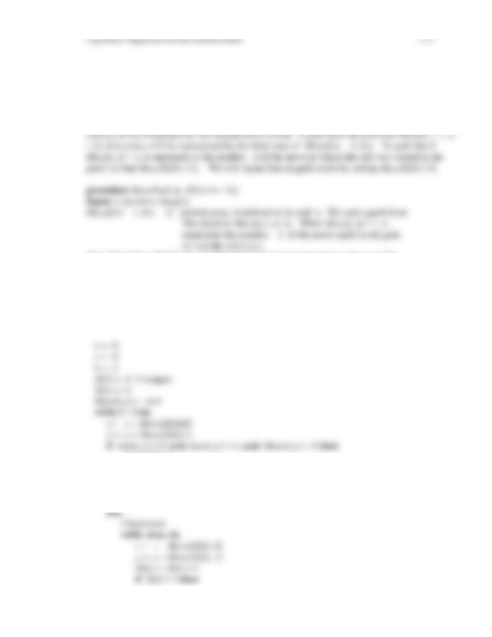
10.5 a.
procedure SumOfSubsets2(A[0:n – 1], Sum, X[0:n])
Input: A[0:n – 1] (an array of positive integers)
Sum (a positive integer)
X[0:n] (an array of integers where X[1:n] stores fixed-tuple
if Temp < Sum then
X[k] ← 1 //visit left child of E-node
PathSum ← Temp
else
Algorithms: Sequential, Parallel and Distributed, Second Edition 10-5
k ← k – 1
endwhile
if k = 0 then return endif
X[k] ← 0
PathSum ← PathSum – A[k – 1]
tuple problem states, X[1],…,X[k] have already been assigned,
and where X[0] = – 1 for convenience of pseudocode)
PathSum (global variable = A[0]*[X[1]] + … + A[k – 1]*[X[k]])
Output: print all descendant goal states of (X[1],…,X[k]); that is, print all
(X[1],…,X[k],X[k+1],…,X[n]) such that A[0]*[X[1]] + … + A[k – 1]*[X[k]]) + A[k]*X[k+1]
else
SumOfSubsetsRec(k)
endif
endfor
end SumOfSubsetsRec2
10.7 In procedure Backtrack, the statements
if (X[1], … , X[k]) is a goal state then
Print(X[1], … , X[k])
endif
if .not. Bounded(X[1], … , X[k]) then
10.8 Similar to how procedure BacktrackRecMin was obtained by modifying BacktrackRec, to
obtain BacktrackMin, we add an output parameter CurrentBest to procedure Backtrack,
which is initialized to ∞. We then modify the statement
if (X[1], … , X[k]) is a goal state then

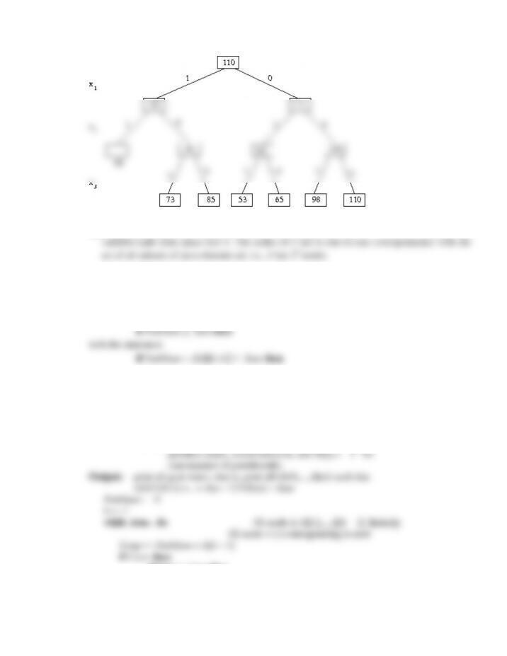
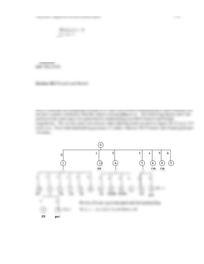
10.9 The following is the portion of the variable-tuple state-space for the instance of the 0/1
knapsack problem given in Exercise 10.1 using the bounding functions (10.2.5) and (10.2.8)
in the text.
110
85
65
98
103
104
100
105
49.5 74.75 82 89
55.7 63.4 67.7 71.3 LoBd=105
SB DB DB DB leaf
55.7 59.9 49.5 52 56.1
DB SB leaf
62
55.7 61 SB leaf SB/DB SB leaf
SB leaf Optimal
3 4 5 6
73
66
60
61
67
78
79
75
80
53
58
59
60
10.10 a.
In the following pseudocode for 0/1-Knapsack, we assume the variable-tuple state-space tree,
and that V[0]/W[0] ≥ V[1]/W[1] ≥ … ≥ V[n – 1]/W[n – 1] in order to conveniently apply the
greedy solution when computing a lower bound on a problem state. We also assume that W[0]
+ W[1] + … + W[n – 1] ≥ C, otherwise all the objects fit in the knapsack, and the solution is
X[0:n] (an array of integers where X[1:n] stores the variable-tuple
problem states, and X[0] = – 1 for convenience of pseudocode)
Output: Best = (X[1],…,X[k – 1]) (an optimal solution)
Weight ← 0
UB ← ∞
//corresponding to root
ChildSearch ← .true.
while ChildSearch do //searching for unbounded child of E-node
if X[k] = – 1 then
X[k] ← X[k – 1] + 1 //visit first child of E-node
LeftOutValue ← LeftOutValue – V[X[k]]
if Weight ≤ C then //(X[1],…,X[k]) is not statically bounded
if LeftOutValue < UB then //update best solution found so far
UB ← LeftOutValue
CurrentBest ← (X[1],…,X[k])
if X[k] > n – 1 then
X[k] ← – 1 //backtrack to previous level; no more children of E-node
k ← k – 1
else
k ← k + 1 //go one more level deep in state space tree
10.12 a. In the following pseudocode for Queens, we use the array Diag1 to index the
diagonals of the board Board[0:n – 1, 0:n – 1] where points Board[i, j] on the diagonal have
i increasing with j , and where we use the array Diag2 to index the diagonals where i
increases opposite to j. The array Vert indexes the columns.
procedure Queens(n)
Board[k,Next[k]] ← 0
Vert[Next[k]] ← 0
Diag1[k – Next[k] + n – 2] ← 0
Diag2[k + Next[k] – 1] ← 0
Next[k] ← Next[k] + 1
PrintBoard(Board,n) //print out the board
Board[k,Next[k]] ← 0
Vert[Next[k]] ← 0
Diag1[k – Next[k] + n – 2] ← 0
Diag2[k + Next[k] – 1] ← 0
else // not in last row
k ← k + 1 // go to next row in board
endif
else // continue looking for place for queen in row k
Next[k] ← Next[k] + 1
10.13 a.
In the following pseduocode for Knight’sTour, Move[0:7, 0:1] has been initialized to represent
the 8 pairs (1,2), (1,-2), (-1,2), (-1,-2), (2,1), (2,-1), (-2,1), (-2,-1), which represent the possible
displacements for a knight’s move from a given cell (p,q) in Board[0:n – 1, 0:n – 1]. Hence,
from (p,q), the knight can move to the cell (p + Move[i,0], q + Move[i,1]), i = 0, 1, …, 7 in

Board[0:n – 1, 0:n – 1] (global array, initialized to – 1s)
Output: a knight’s starting at Board[x,y], where Board[x,y] = – 1 signals that no such knight’s
tour exists.
Board[0:n – 1, 0:n – 1] (when tour exists, Board[p, q] represents the number of the
move made by the knight to visit the cell (p,q) starting
if min(x, y) ≥ 0 .and. max(x,y) < n .and. Board[x,y] = – 1 then
// good move
k ← k + 1;
Board[x,y] ← k;
if k = n*n then return endif // found the tour
else
break
endif
endwhile
endif
10.14 a.
In the following pseduocode for MazePath, Move[0:3, 0:1] has been initialized to represent the
4 pairs (1,0), (-1,0), (0,1), (0,-1), which represent the possible displacements for a move to an
adjacent cell in Maze[0:n – 1, 0:n – 1]. Hence, from cell (p,q), a move can be made to the cell
(p + Move[i,0], q + Move[i,1]), i = 0, 1, 2,3 in Maze [0:n – 1, 0:n – 1] so long as a given such
Move[0:3, 0:1] (global array initialized to 4 displacements representing possible
moves in the maze)
Output: Maze[0:n – 1, 0:n – 1], and when a path exists, if Maze[p,q] > 1, it represents the
number of the moves – 2 made to get to the cell [p,q]. When Maze[0,0] = 0, then no path
exists. X[0:n*n – 1] where X[k] contains a move made in kth point in the path.
// good move
k ← k + 1
Maze[x,y] ← k+1
if x = n – 1 .and. y = n – 1 then return endif // found the path
X[k] ← 0
else
break
endif
endwhile
endif
10.16 For this problem we use the variable-tuple state-space tree, and we incorporate the
improvement to SumOfSubsetsMin discussed on p. 311 in the text. This improvement results from
the fact that we only want a single optimal goal. Hence, when a goal X is generated, there is no
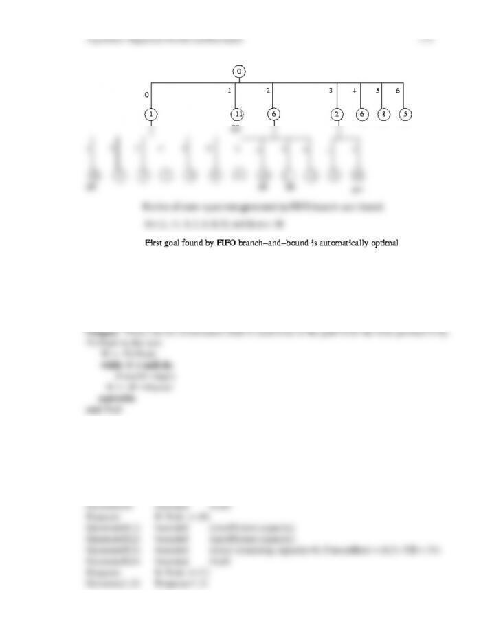
10.17 All that is required is to put a return statement after the Path(Child) statement.
10.18
procedure Path(PtrNode)
Input: PtrNode (pointer to node in parent representation of state-space tree)
10.19
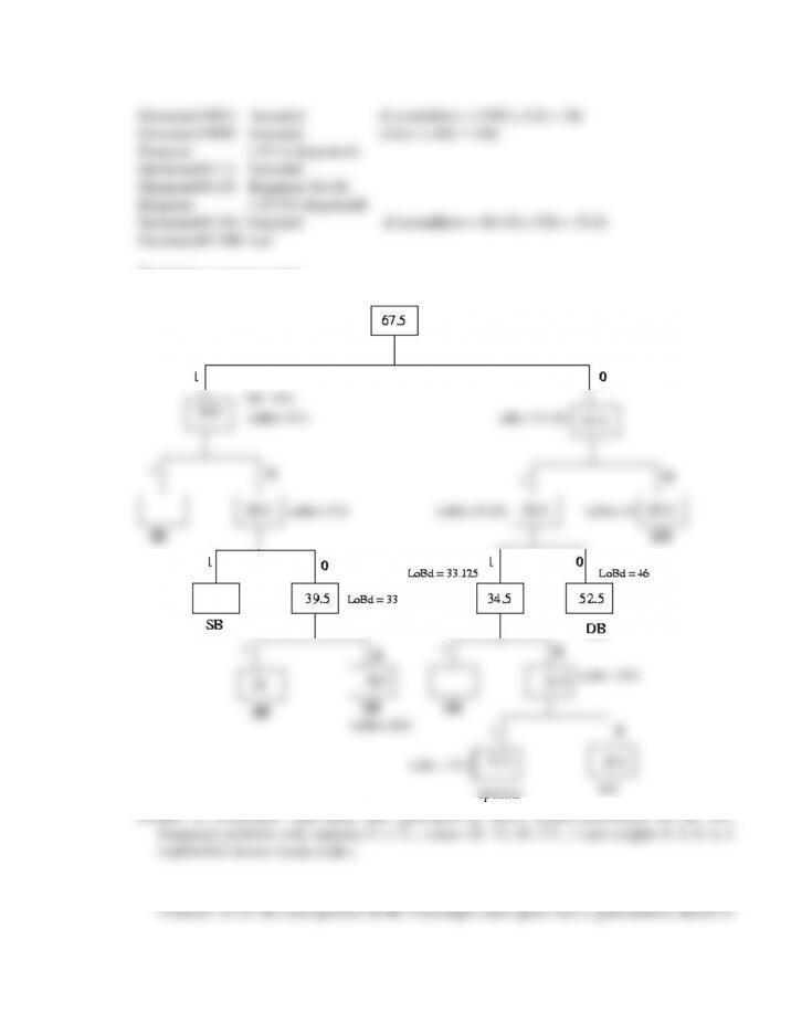
Generate(0) Enqueue(0) (CurrentBest = (0), UB = 39.5)
Generate(1) Enqueue(1)
Generate(2) bounded (since LoBd > UB)
Generate(3) bounded (since LoBd > UB)

67.5
UB = 39.5 0 UB = 39.5 1 UB=39.5 2 UB=39.5 3 UB=39.5 4
39.5
52.5
49.5
LoBd= LoBd= LoBd =
33.125 DB 46
leaf 51.5
SB leaf Optimal
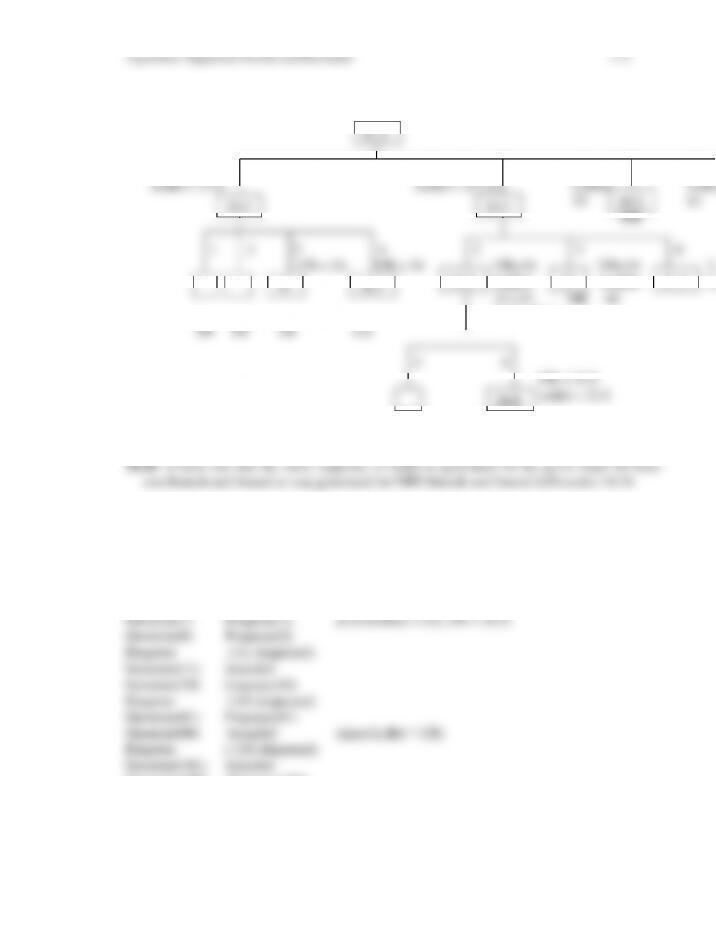
10.21 When discussing generating problem states for the fixed-tuple state-space tree for the
given problem, we will use 0/1 sequences to denote the path from the root to the given problem
state, with 1 indicating that we are using the corresponding element (left child), and 0 indicated
that we are not. For example, the problem state (1,0,0,1) corresponds to choosing the elements
with values 28 and 5.5, and not choosing the elements with values 15 and 18.
Generate(100) Enqueue(100)
Dequeue ( (01) dequeued)
Generate(011) Enqueue(011) (CurrentBest = (011), UB = 34.5)
Generate(010) bounded (since LoBd > UB)
Dequeue ( (100) dequeued)
34
38.5
34.5
47
51.5
33.5
Algorithms: Sequential, Parallel and Distributed 1-18
Terminate on queue empty
10.22 Using least-cost branch-and-bound for the same input to the 0/1 Knapsack problem as in
Exercise 10.21 for FIFO branch-and-bound. However, the nodes are generated in a different
sequence, as shown below.
Generate(1) Enqueue(1) (CurrentBest = (1), UB = 39.5, LoBd = 27.5)
Generate(0) Enqueue(0) (LoBd = 33.125)
Dequeue ( (1) dequeued)