Chapter 8 Linear Programming Methods for Optimum Design
Arora, Introduction to Optimum Design, 4e
8-21
8.29 ________________________________________________________________________________
Find all the basic solutions for the following LP problem using the Gauss-Jordan elimination
method. Identify basic feasible solutions and show them on graph paper.
Maximize = 41+ 22
Subject to −21+2≤4
1+ 22≥2
1,2≥0
Solution:
Standard LP form:
Table 8.29
1
2
3
4
f
1.
0
0
4
-2
0
infeasible
2.
0
4
0
6
-8
feasible
3.
0
1
3
0
-2
feasible
4.
-2
0
0
-4
8
infeasible
5.
2
0
8
0
-8
feasible
6.
-1.2
1.6
0
0
1.6
infeasible
Chapter 8 Linear Programming Methods for Optimum Design
8.30 ________________________________________________________________________________
Find all the basic solutions for the following LP problem using the Gauss-Jordan elimination
method. Identify basic feasible solutions and show them on graph paper.
Maximize = 31+ 22
Subject to 1− 2≥0
1+2≥2
1,2≥0
Solution:
Standard LP form:
Table E8.30
1
2
3
4
f
1.
0
0
0
-2
0
infeasible
2.
0
0
0
-2
0
infeasible
3.
0
2
-2
0
-4
infeasible
4.
0
0
0
-2
0
infeasible
5.
2
0
2
0
-6
feasible
6.
1
1
0
0
-5
feasible
Chapter 8 Linear Programming Methods for Optimum Design
Arora, Introduction to Optimum Design, 4e
8-23
8.31 ________________________________________________________________________________
Find all the basic solutions for the following LP problem using the Gauss-Jordan elimination
method. Identify basic feasible solutions and show them on graph paper.
Maximize = 41+ 52
Subject to −1+ 22≤10
31+ 22≤18
1,2≥0
Solution:
Standard LP form:
Table E8.31
1
2
3
4
f
1.
0
0
10
18
0
feasible
2.
0
5
0
8
-25
feasible
3.
0
9
-8
0
-45
infeasible
4.
-10
0
0
48
40
infeasible
5.
6
0
16
0
-24
feasible
6.
2
6
0
0
-38
feasible
Chapter 8 Linear Programming Methods for Optimum Design
Section 8.5 The Simplex Method
8.32 ________________________________________________________________________________
Solve the following problem by the Simplex method and verify the solution graphically whenever
possible.
Maximize =1+ 0.52
Subject to 61+ 52≤30
31+2≤12
1+ 32≤12
1,2≥0
Solution:
Standard LP form:
Table E8.32
Basic
1
2
3
4
5
b ratio
3
6 5 1 0 0 30
30
6= 5
4
12
3=
5
12
1=12
Cost -1 -0.5 0 0 0 f-0
3
0 3 1 -2 0 6
6
3=
1
1 1/3 0 1/3 0 4
4
1/3=12
5
8
2
5
Arora, Introduction to Optimum Design, 4e
8-25
8.33________________________________________________________________________________
Solve the following problem by the Simplex method and verify the solution graphically whenever
possible.
Maximize = 31+ 22
Subject to 31+ 22≤6
−41+ 92≤36
1,2≥0
Solution:
Standard LP form:
Table E8.33
Basic
1
2
3
4
b ratio
3
3 2 1 0 6
6
3=
4
1
1 2/3 1/3 0 2
2
2/3=
4
44
If
2
is introduced into the basic set, we get the other solution as
2
3/2 1 1/2 0 3
4
Chapter 8 Linear Programming Methods for Optimum Design
8.34 ________________________________________________________________________________
Solve the following problem by the Simplex method and verify the solution graphically whenever
possible.
Maximize =1+ 22
Subject to −1+ 32≤10
1+2≤6
1− 2≤2
1,2≥0
Solution:
Table E8.34
Basic
1
2
3
4
5
b ratio
3
4
5
Cost –1 -2 0 0 0 f-0
2
-1/3 1 1/3 0 0 10/3 negative
4
5
2
0 1 1/4 1/4 0 4
1
1 0 -1/4 3/4 0 2
5
Arora, Introduction to Optimum Design, 4e
8-27
8.35 ________________________________________________________________________________
Solve the following problem by the Simplex method and verify the solution graphically whenever
possible.
Maximize = 21+2
Subject to −1+ 22≤10
31+ 22≤18
1,2≥0
Solution:
Standard LP form:
Table E8.35
Basic
1
2
3
4
b ratio
3
-1 2 1 0 10 negative
4
18
3
0 8/3 1 1/3 16
1
Chapter 8 Linear Programming Methods for Optimum Design
8.36 ________________________________________________________________________________
Solve the following problem by the Simplex method and verify the solution graphically whenever
possible.
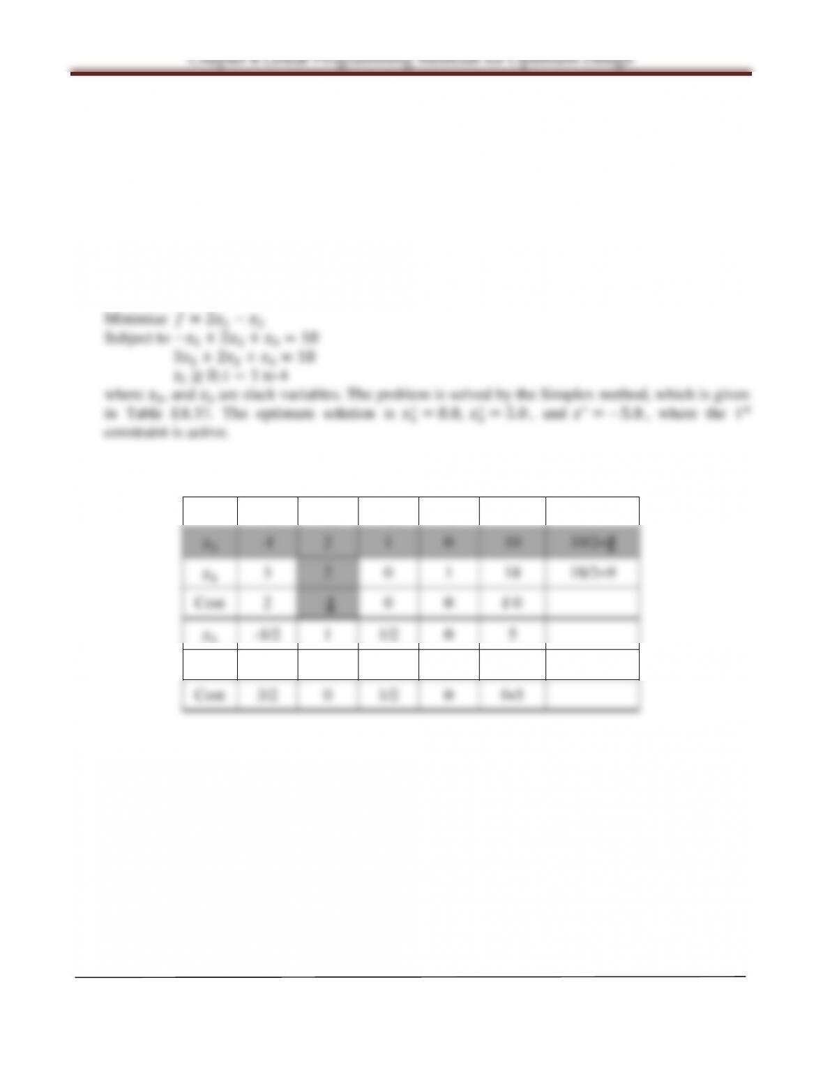
Maximize = 51−22
Subject to 21+2≤9
1− 2≤2
−31+ 22≤3
1,2≥0
Solution:
Standard LP form:
Table E8.36
Basic
1
2
3
4
5
b ratio
3
4
5
3
0 3 1 -2 0 5 5/3
1
5
2
1
1 0 1/3 1/3 0 11/3
5
Arora, Introduction to Optimum Design, 4e
8-29
8.37 ________________________________________________________________________________
Solve the following problem by the Simplex method and verify the solution graphically whenever
possible.
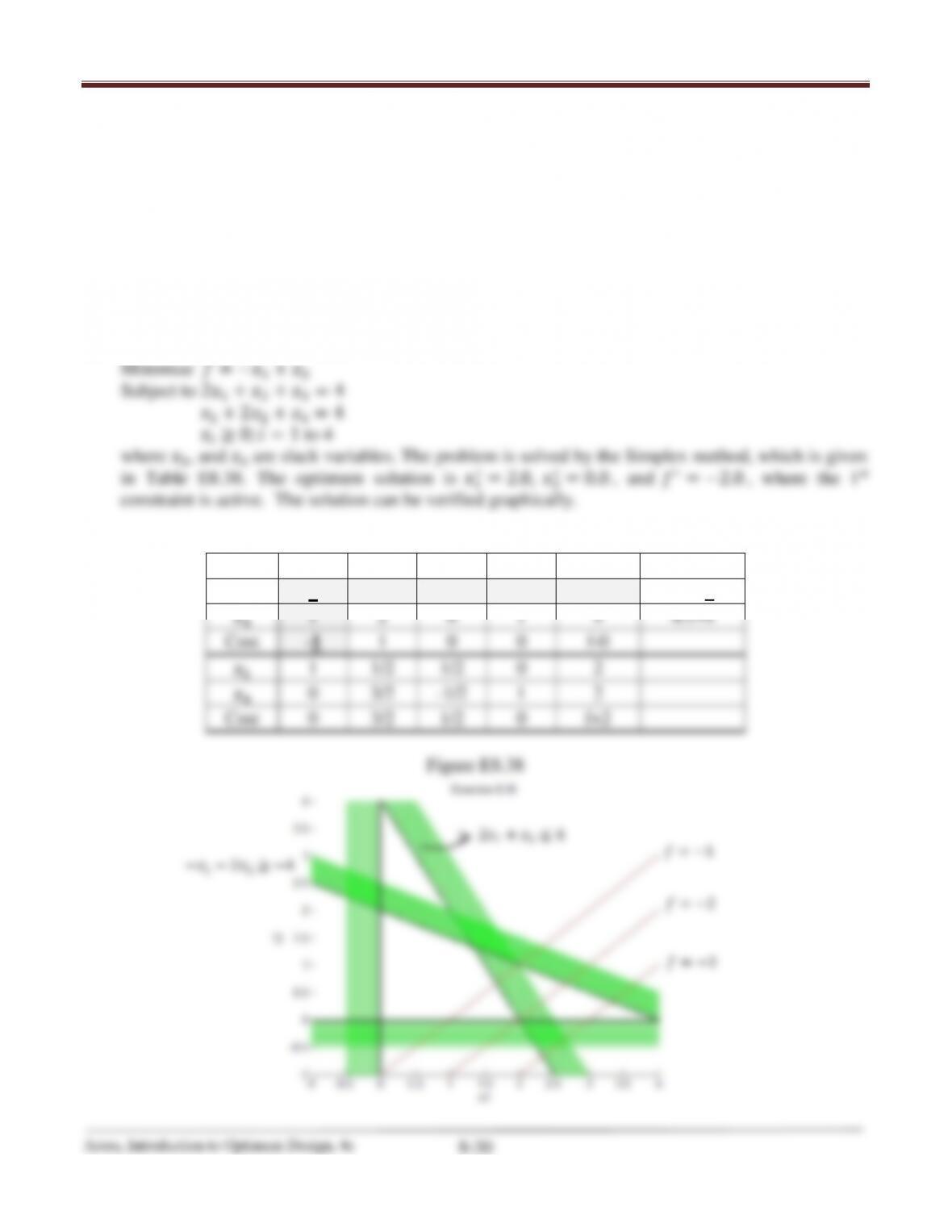
Minimize = 21− 2
Subject to −1+ 22≤10
31+ 22≤18
1,2≥0
Solution:
Standard LP form:
Table E8.37
Basic
1
2
3
4
b ratio
3
4
4
4 0 -1 1 8
Chapter 8 Linear Programming Methods for Optimum Design
8.38 ________________________________________________________________________________
Solve the following problem by the Simplex method and verify the solution graphically whenever
possible.
Minimize =−1+2
Subject to 21+2≤4
−1−22≥ −4
1,2≥0
Solution:
Standard LP form:
Table E8.38
Basic
1
2
3
4
b
ratio
3
2
1
1
0
4
4/2=2
4
1
2
0
1
4
4/1=4
Cost
–1
1
0
0
f-0
1
1
1/2
1/2
0
2
4
0
3/2
-1/2
1
2
Cost
0
3/2
1/2
0
f+2
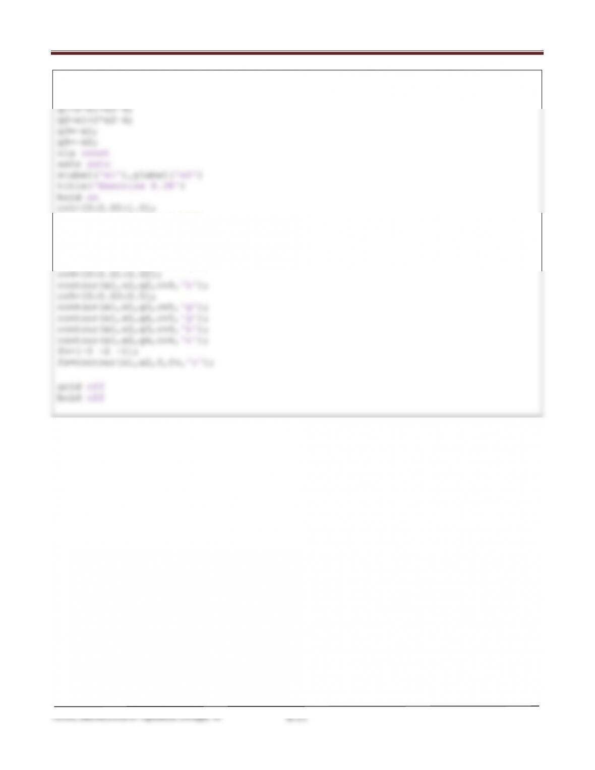
Figure E8.38
−1−22≥ −4
21+2≤4
=−1
=−2
=−3
Chapter 8 Linear Programming Methods for Optimum Design
clear all
[x1,x2]=meshgrid(-1:0.05:4, –1:0.05:4);
f=–x1+x2;
contour(x1,x2,g1,cv1,‘g’);
cv2=[0:0.01:0.02];
contour(x1,x2,g1,cv2,‘k’);
cv3=[0:0.05:1.0];
contour(x1,x2,g2,cv3,‘g’);
8.39 __________________________________________________________________________
Solve the following problem by the Simplex method and verify the solution graphically whenever
possible.
Maximize = 21− 2
Subject to 1+ 22≤6
2≥ 1
1,2≥0
Solution
Standard LP form:
Table E8.39
Basic
1
2
3
4
b
ratio
3
1
2
1
0
6
6/1=6
4
1
0
0
1
2
2/1=2
Cost
-2
1
0
0
f-0
3
0
2
1
-1
4
1
1
0
0
1
2
Cost
0
1
0
2
f+4
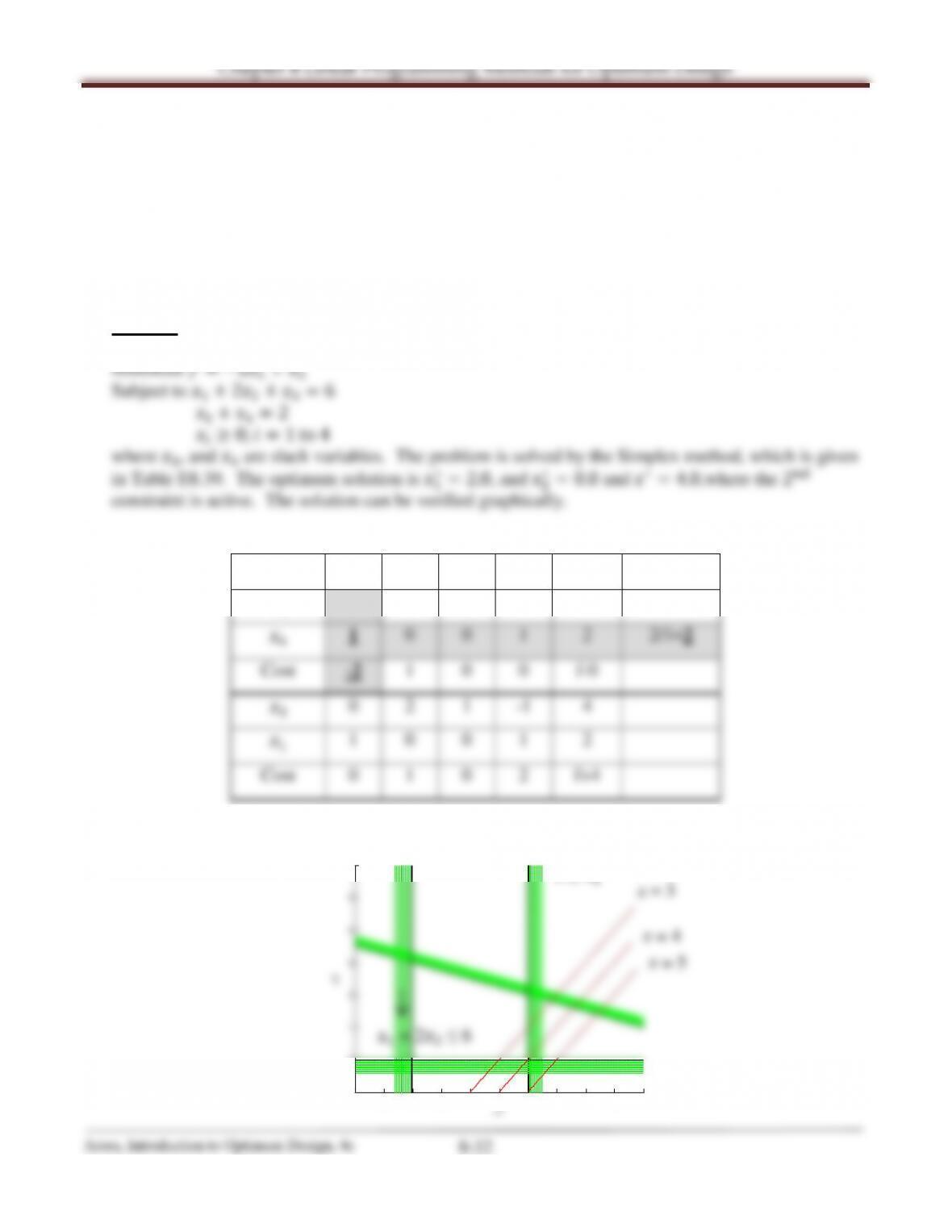
Figure E8.39
-1 -0.5 00.5 11.5 22.5 33.5 4
-1
0
1
2
3
4
5
6
x2
Ex ercise 8.39
z = 3
z = 4
z = 5
2 ≥ x1
x1 + 22 ≤ 6
Chapter 8 Linear Programming Methods for Optimum Design
clear all
[x1,x2]=meshgrid(–1:0.05:4, –1:0.05:6);
f=–2*x1+x2;
g1=x1+2*x2–6;
g2=x1–2;
g3=–x1;
g4=–x2;
cla reset
axis auto
xlabel(‘x1’),ylabel(‘x2’)
title(‘Exercise 8.39’)
hold on
cv1=[0:0.04:0.6];
contour(x1,x2,g1,cv1,‘g’);
cv2=[0:0.01:0.02];
contour(x1,x2,g1,cv2,‘k’);
cv3=[0:0.02:0.25];
contour(x1,x2,g2,cv3,‘g’);
cv4=[0:0.01:0.01];
contour(x1,x2,g2,cv4,‘k’);
cv5=[0:0.025:0.3];
grid off;
hold off;
Arora, Introduction to Optimum Design, 4e
8-34
8.40 ________________________________________________________________________________
Solve the following problem by the Simplex method and verify the solution graphically whenever
possible.
Maximize =1+2
Subject to 41+ 32≤12
1+ 22≤4
1,2≥0
Solution:
Standard LP form:
Table E8.40
Basic
1
2
3
4
b ratio
3
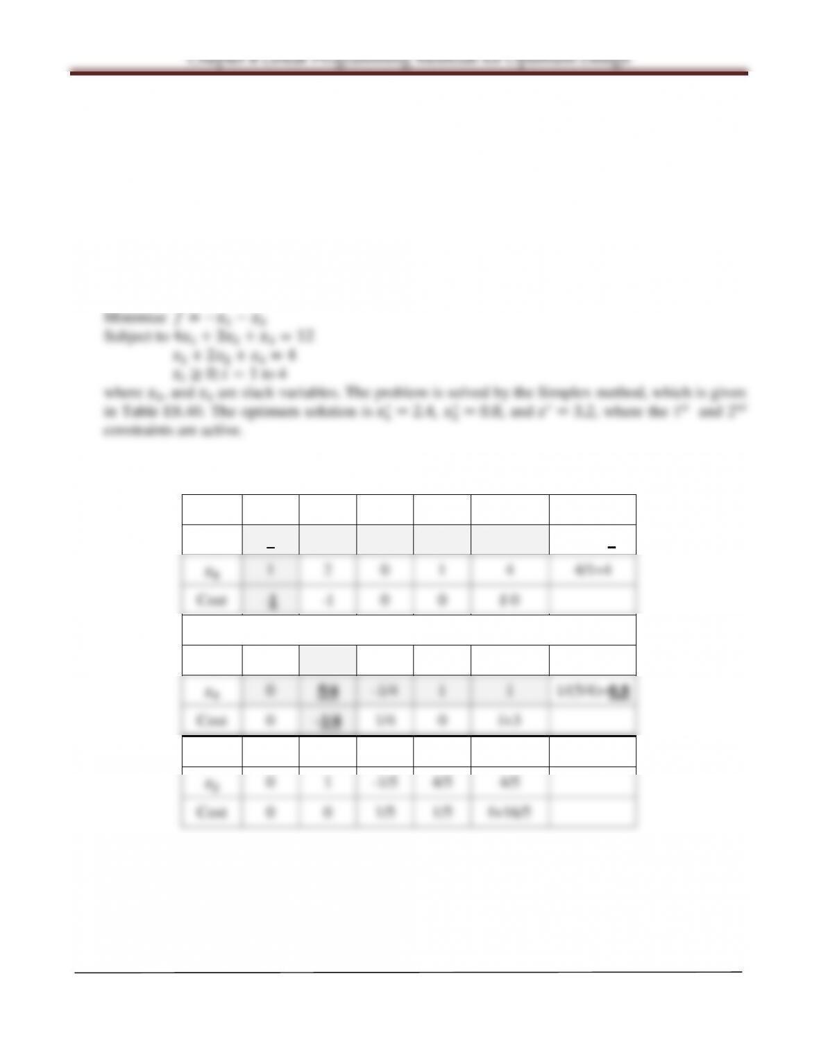
4 3 1 0 12 12/4=3
4
If
1
is introduced into the basic set, we get the other solution as
1
1 3/4 1/4 0 3 3/¾=4
4
1
1 0 2/5 -3/5 12/5
2
Chapter 8 Linear Programming Methods for Optimum Design
8.41 ________________________________________________________________________________
Solve the following problem by the Simplex method and verify the solution graphically whenever
possible.
Maximize =−21+2
Subject to 1≤2
1+ 22≤6
1,2≥0
Solution:
Standard LP form:
Table E8.41
Basic
1
2
3
4
b ratio
3
1 0 1 0 2 ∞
4
2
Arora, Introduction to Optimum Design, 4e
8-36
8.42 ________________________________________________________________________________
Solve the following problem by the Simplex method and verify the solution graphically whenever
possible.
Maximize = 21+2
Subject to 41+ 32≤12
1+ 22≤4
1,2≥0
Solution:
Standard LP form:
Table E8.42
Basic
1
2
3
4
b ratio
3
4 3 1 0 12 12/4=3
4
1
4
1
1 0 1 -2 0
2
Chapter 8 Linear Programming Methods for Optimum Design
8.43 ________________________________________________________________________________
Solve the following problem by the Simplex method and verify the solution graphically whenever
possible.
Minimize = 91+ 22+ 33
Subject to 21+2−33≥ −5
−1−22+ 23≥ −2
1,2,3≥0
Solution:
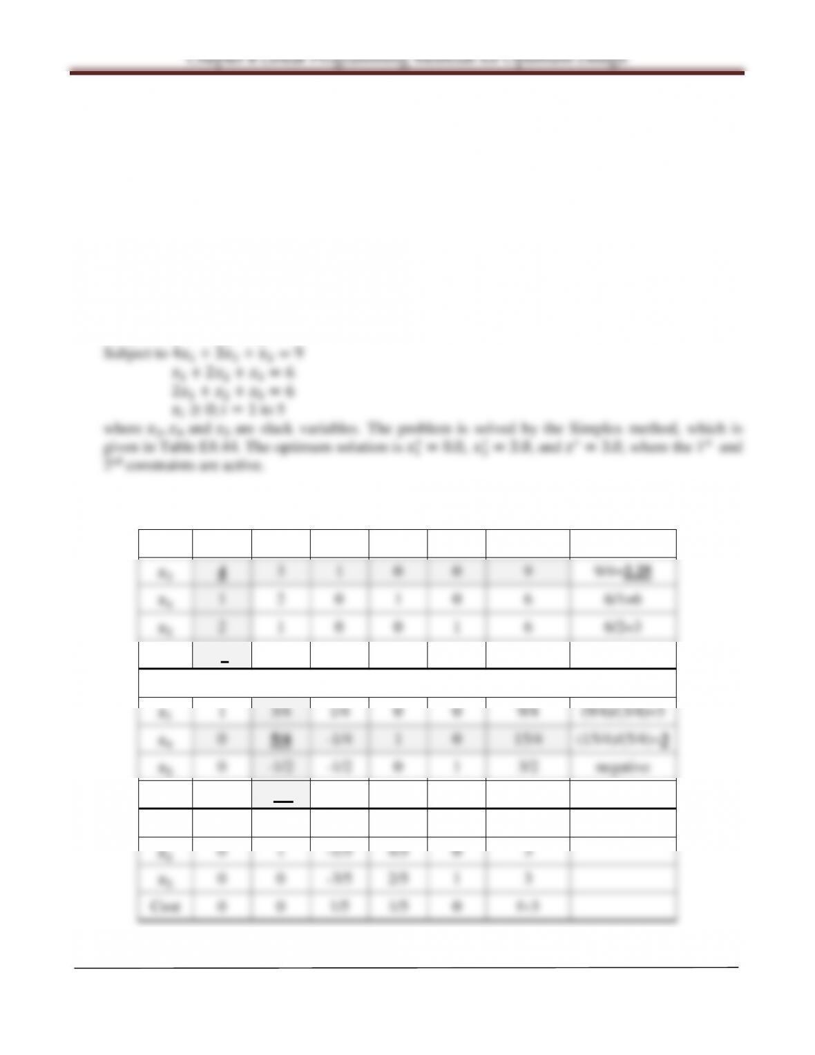
Standard LP form:
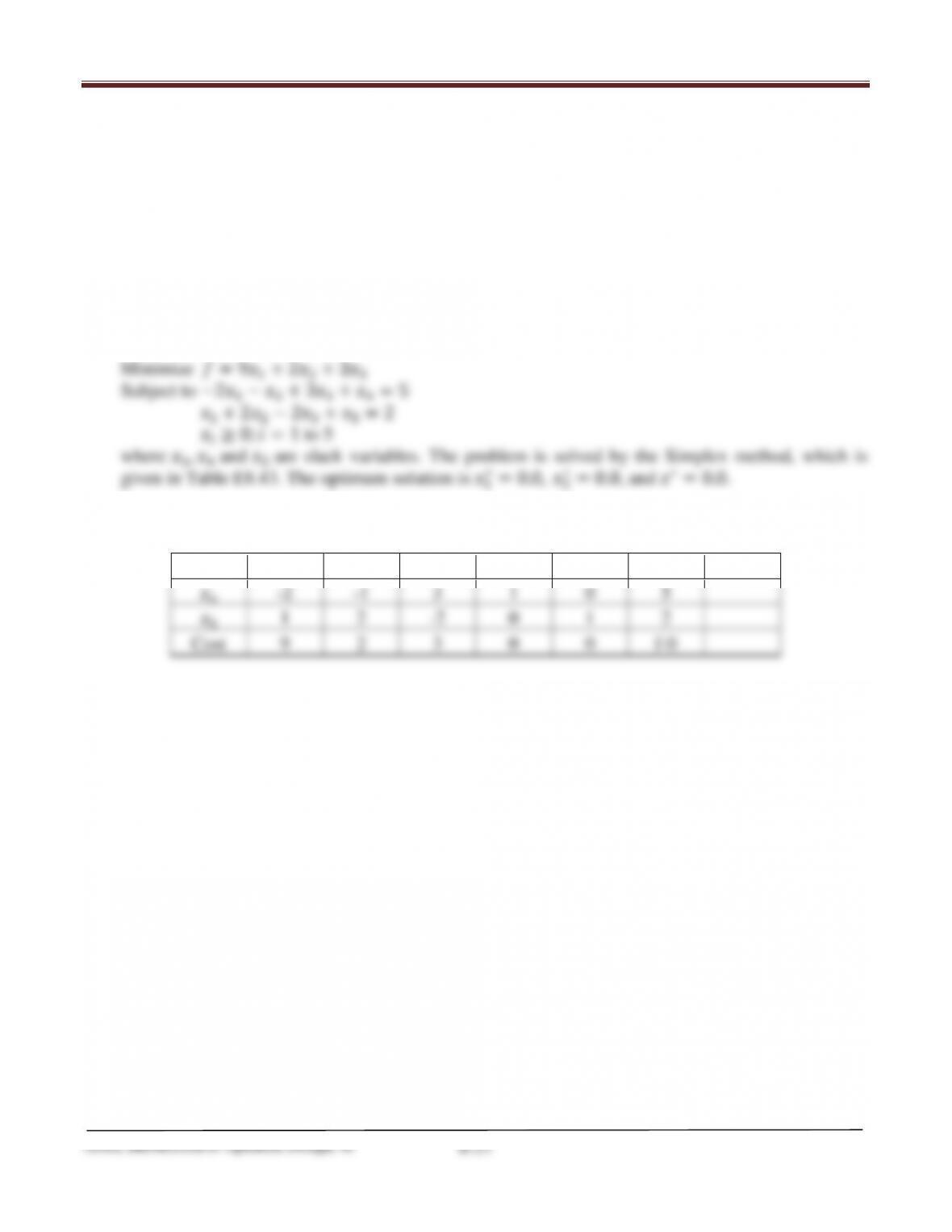
given in Table E8.43. The optimum solution is 1
Table E8.43
Basic
1
2
3
4
5
b
ratio
4
-2
-1
3
1
0
5
5
1
2
-2
0
1
2
Cost
9
2
3
0
0
f-0
Arora, Introduction to Optimum Design, 4e
8-38
8.44 ________________________________________________________________________________
Solve the following problem by the Simplex method and verify the solution graphically whenever
possible.
Maximize =1+2
Subject to 41+ 32≤9
1+ 22≤6
21+2≤6
1,2≥0
Solution:
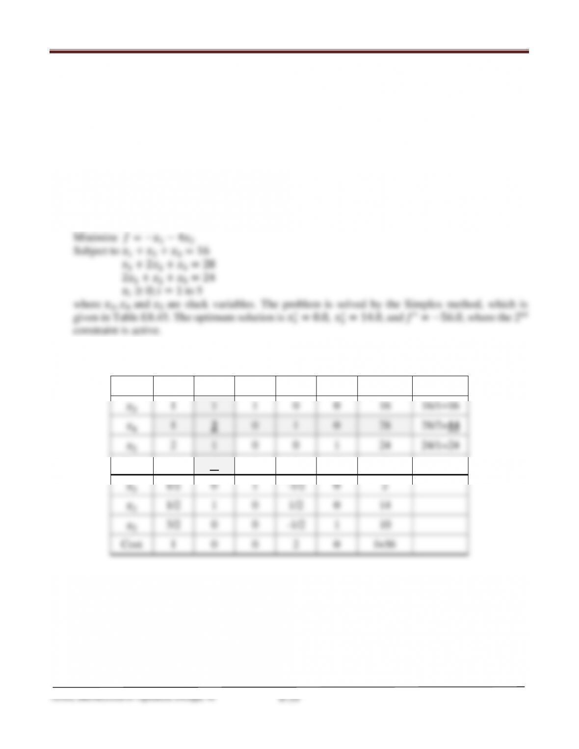
Standard LP form:
Minimize =−1− 2
Table E8.44
Basic
1
2
3
4
5
b ratio
3
4
5
Cost –1 -1 0 0 0 f-0
If
1
is introduced into the basic set, we get the other solution as
1
4
5
Cost 0 –1/4 1/4 0 0 f+9/4
1
1 0 2/5 -3/5 0 0
2
5
Chapter 8 Linear Programming Methods for Optimum Design
8.45 ________________________________________________________________________________
Solve the following problem by the Simplex method and verify the solution graphically whenever
possible.
Minimize =−1−42
Subject to 1+2≤16
1+ 22≤28
24 ≥21+2
1,2≥0
Solution:
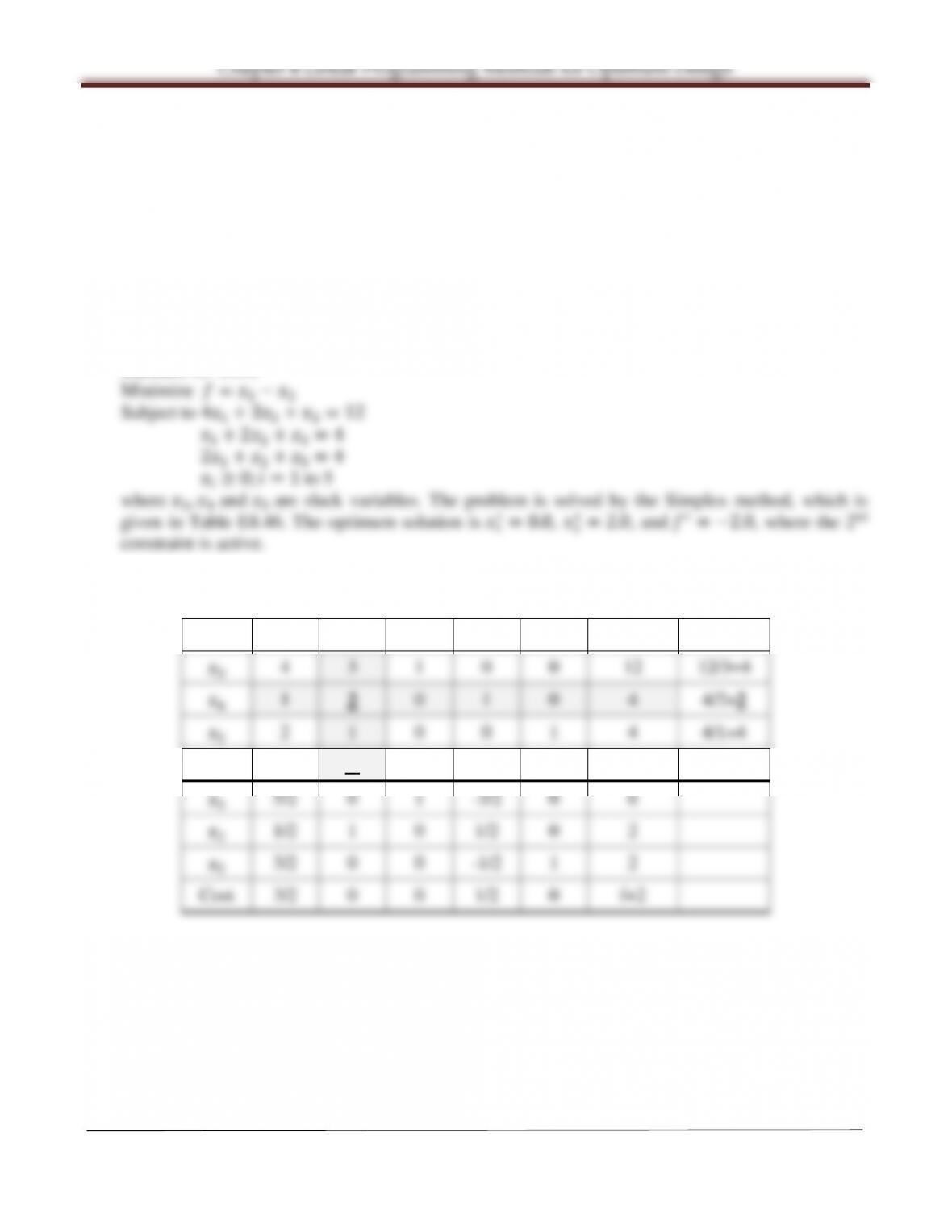
Standard LP form:
Table E8.45
Basic
1
2
3
4
5
b ratio
3
1 1 1 0 0 16 16/1=16
4
1 2 0 1 0 28 28/2=14
5
2 1 0 0 1 24 24/1=24
Cost -1 -4 0 0 0 f
3
1/2 0 1 -1/2 0 2
2
1/2 1 0 1/2 0 14
5
3/2 0 0 -1/2 1 10
Cost 1 0 0 2 0 f+56
Arora, Introduction to Optimum Design, 4e
8-40
8.46 ________________________________________________________________________________
Solve the following problem by the Simplex method and verify the solution graphically whenever
possible.
Minimize =1− 2
Subject to 41+ 32≤12
1+ 22≤4
4≥21+2
1,2≥0
Solution:
Standard LP form:
Table E8.46
Basic
1
2
3
4
5
b ratio
3
4 3 1 0 0 12 12/3=4
4
1 2 0 1 0 4 4/2=2
5
2 1 0 0 1 4 4/1=4
Cost 1 -1 0 0 0 f
3
5/2 0 1 -3/2 0 6
2
1/2 1 0 1/2 0 2
5
3/2 0 0 -1/2 1 2
Cost 3/2 0 0 1/2 0 f+2