Arora, Introduction to Optimum Design, 4e
8-41
8.47 ________________________________________________________________________________
Solve the following problem by the Simplex method and verify the solution graphically whenever
possible.
Maximize = 21+ 32
Subject to 1+2≤16
−1−22≥ −28
24 ≥21+2
1,2≥0
Solution:
Standard LP form:
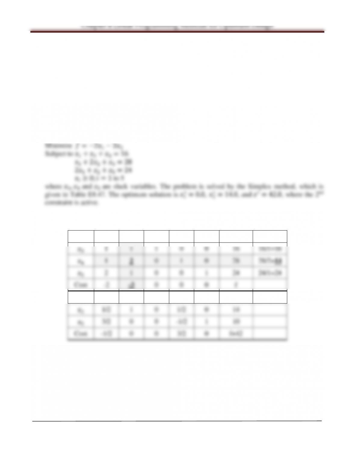
Table E8.47
Basic
1
2
3
4
5
b ratio
3
4
5
3
1/2 0 1 -1/2 0 2
2
5
Chapter 8 Linear Programming Methods for Optimum Design
8.48 ________________________________________________________________________________
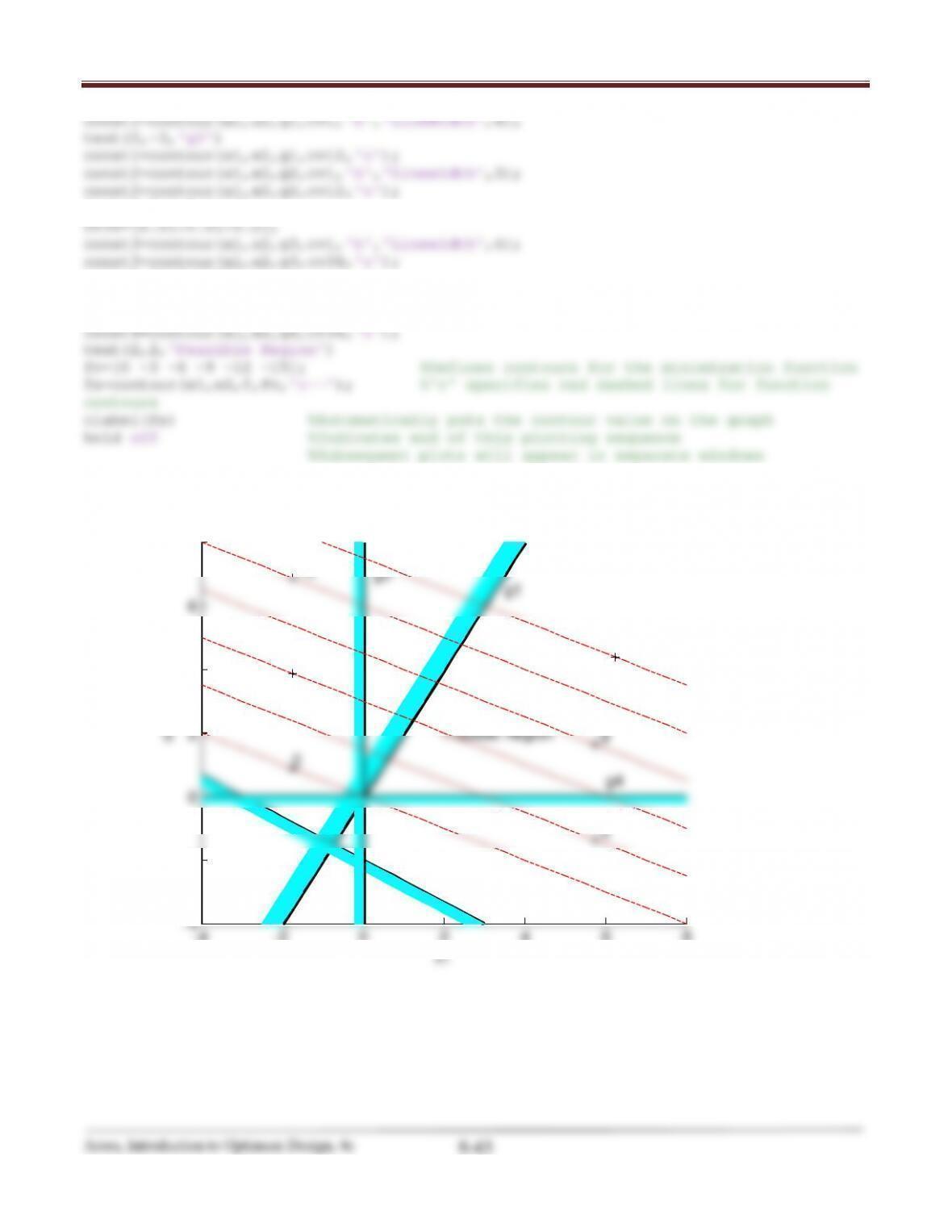
Solve the following problem by the Simplex method and verify the solution graphically whenever
possible.
Maximize =1+ 22
Subject to 21− 2≥0
21+ 32≥ −6
1,2≥0
Solution:
Standard LP form:
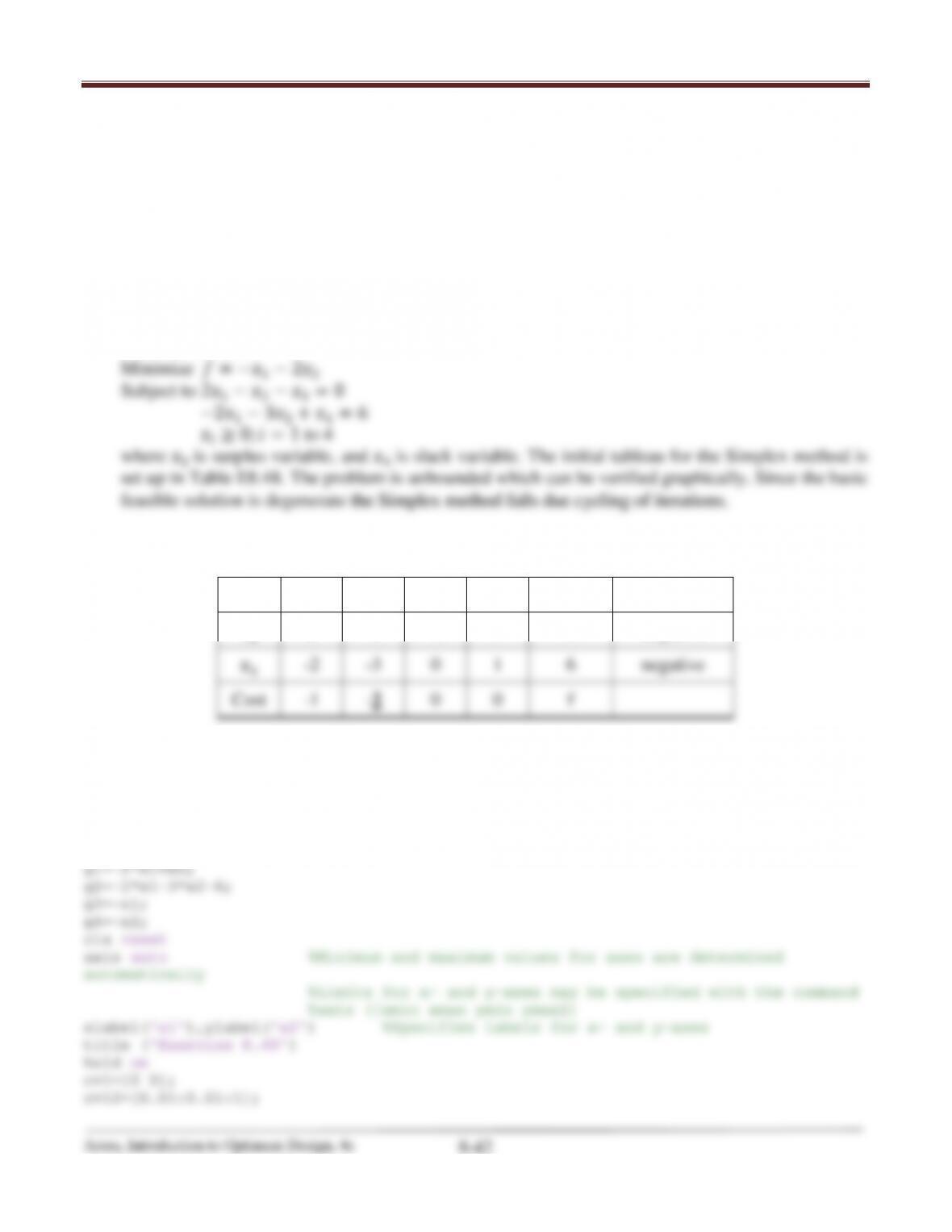
Table E8.48
Basic
1
2
3
4
b ratio
3
2 -1 -1 0 0 negative
4
Matlab Code
%Exercise 8.48
%Create a grid from –4 to 8 with an increment of 0.5 for the variables x1 and x2
[x1,x2]=meshgrid(–4:0.5:8.0, –4:0.5:8.0);
%Enter functions for the minimization problem
f=–x1–2*x2;
Chapter 8 Linear Programming Methods for Optimum Design
const1=contour(x1,x2,g1,cv1,‘k’,‘LineWidth’,4);
text(2,–3,‘g2’)
const1=contour(x1,x2,g1,cv12,‘c’);
const2=contour(x1,x2,g2,cv1,‘k’,‘Linewidth’,3);
const2=contour(x1,x2,g2,cv12,‘c’);
text(3.5,6.5,‘g1’)
text(0.25,7,‘g3’)
const4=contour(x1,x2,g4,cv1,‘k’,‘LineWidth’,3);
text(6,0.5,‘g4’)
0
2
4
6
8
x2
Exercise 8.48
g1
g3
g4
Feasible Region
–15
–12
-9
-6
-3
0
Chapter 8 Linear Programming Methods for Optimum Design
8.49 ________________________________________________________________________________
Solve the following problem by the Simplex method and verify the solution graphically whenever
possible.
Maximize = 21+ 22+3
Subject to 101+ 93≤375
1+ 32+3≤33
2≥ 3
1,2,3≥0
Solution:
Standard LP form:
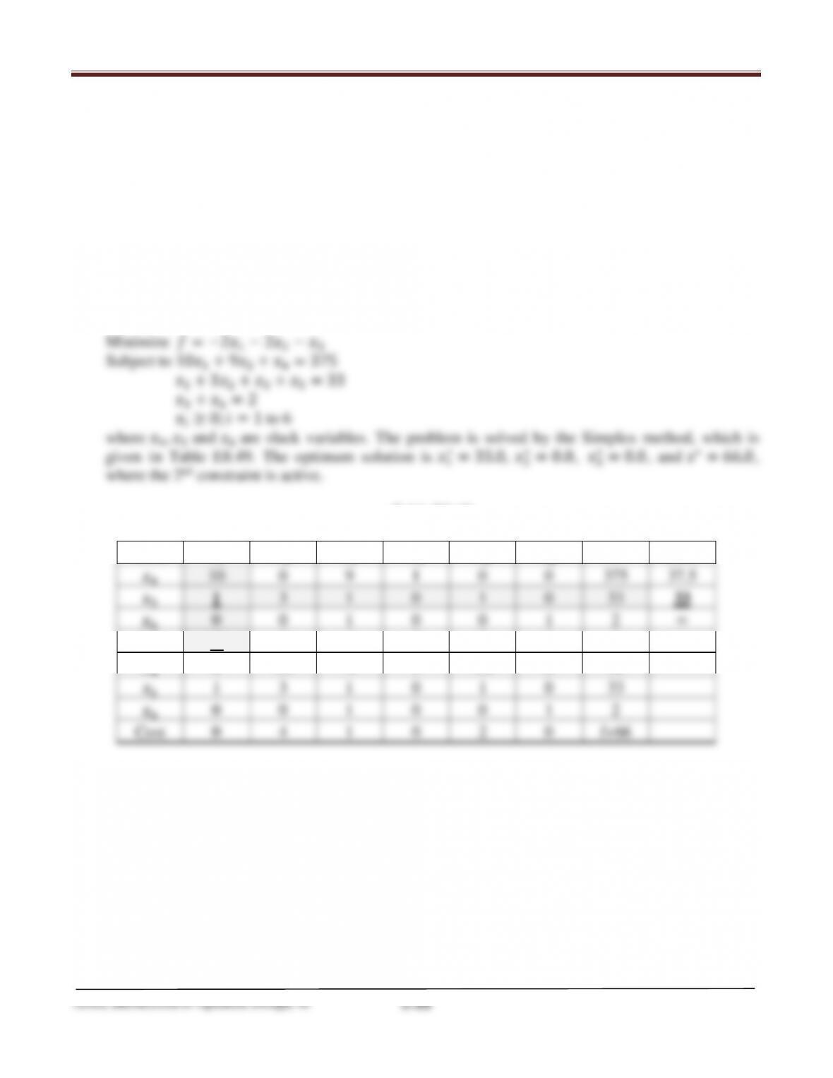
Table E8.49
Basic
1
2
3
4
5
6
b
ratio
4
10
0
9
1
0
0
375
37.5
5
1
3
1
0
1
0
33
33
6
0
0
1
0
0
1
2
∞
Cost
-2
-2
-1
0
0
0
f
4
0
-30
-1
1
-10
0
45
1
1
3
1
0
1
0
33
6
0
0
1
0
0
1
2
Cost
0
4
1
0
2
0
f+66
Arora, Introduction to Optimum Design, 4e
8-45
8.50 ________________________________________________________________________________
Solve the following problem by the Simplex method and verify the solution graphically whenever
possible.
Maximize =1+ 22
Subject to −21− 2≥ −5
31+ 42≤10
1≤2
1,2≥0
Solution:
Standard LP form:
Table E8.50
Basic
1
2
3
4
5
b
ratio
3
2
1
1
0
0
5
5/1=5
4
3
4
0
1
0
10
10/4=2.5
5
1
0
0
0
1
2
∞
Cost
-1
-2
0
0
0
f
3
5/4
0
1
-1/4
0
5/2
2
3/4
1
0
1/4
0
5/2
5
1
0
0
0
1
2
Cost
1/2
0
0
1/2
0
f+5
Chapter 8 Linear Programming Methods for Optimum Design
8.51 ________________________________________________________________________________
Solve the following problem by the Simplex method and verify the solution graphically whenever
possible.
Minimize =−21− 2
Subject to −21− 2≥ −5
31+ 42≤10
1≤3
1,2≥0
Solution:
Standard LP form:
Table E8.51
Basic
1
2
3
4
5
b
ratio
3
2
1
1
0
0
5
5/2=2.5
4
3
4
0
1
0
10
10/3=3.3
5
1
0
0
0
1
3
3/1=3
Cost
-2
-1
0
0
0
f
1
1
1/2
0.5
0
0
5/2
2.5/0.5=5
4
0
5/2
-3/2
1
0
5/2
2.5/2.5=1
5
0
-1/2
-1/2
0
1
1/2
negative
Cost
0
0
1
0
0
f+5
f+5
1
1
0
4/5
-1/5
0
2
2
0
1
-3/5
2/5
0
1
5
0
0
-4/5
1/5
1
1
Cost
0
0
1
0
0
f+5
Arora, Introduction to Optimum Design, 4e
8-47
8.52 ________________________________________________________________________________
Solve the following problem by the Simplex method and verify the solution graphically whenever
possible.
Maximize =121+ 72
Subject to 21+2≤5
31+ 42≤10
1≤2
2≤3
1,2≥0
Solution:
Standard LP form:
Table E8.52
Basic
1
2
3
4
5
6
b
ratio
3
2
1
1
0
0
0
5
5/2=2.5
4
3
4
0
1
0
0
10
10/3
5
1
0
0
0
1
0
2
2/1=2
6
0
1
0
0
0
1
3
∞
Cost
-12
-7
0
0
0
0
f-0
3
0
1
1
0
-2
0
1
1/1=1
4
0
4
0
1
-3
0
4
4/4=1
1
1
0
0
0
1
0
2
∞
6
0
1
0
0
0
1
3
3/1=3
Cost
0
-7
0
0
12
0
f+24
2
0
1
1
0
-2
0
1
4
0
0
-4
1
5
0
0
1
1
0
0
0
1
0
2
6
0
0
-1
0
2
1
2
Cost
0
0
7
0
-2
0
f+31
Chapter 8 Linear Programming Methods for Optimum Design
Arora, Introduction to Optimum Design, 4e
8-48
8.53 ________________________________________________________________________________
Solve the following problem by the Simplex method and verify the solution graphically whenever
possible.
Maximize =101+ 82+ 53
Subject to 101+ 93≤375
51+152+ 33≤35
3≥ 3
1,2,3≥0
Solution:
Standard LP form:
Table E8.53
Basic
1
2
3
4
5
6
b
ratio
4
10
0
9
1
0
0
375
375/10=37.5
5
5
15
3
0
1
0
35
35/5=7
6
0
0
1
0
0
1
3
∞
Cost
-10
-8
-5
0
0
0
f
4
0
-30
3
1
-2
0
305
1
1
3
3/5
0
1/5
0
7
6
0
0
1
0
0
1
3
Cost
0
22
1
0
2
0
f+70
Chapter 8 Linear Programming Methods for Optimum Design
Section 8.6 The Two Phase Simplex Method − Artificial Variables
8.54 ________________________________________________________________________________
Answer True or False.
1. A pivot step of the Simplex method replaces a current basic variable with a nonbasic
2. The pivot step brings the design point to the interior of the constraint set. False
3. The pivot column in the Simplex method is determined by the largest reduced cost
4. The pivot row in the Simplex method is determined by the largest ratio of right–side
parameters with the positive coefficients in the pivot column. False
5. The criterion for a current basic variable to leave the basic set is to keep the new solution
6. A move from one basic feasible solution to another corresponds to extreme points of the
7. A move from one basic feasible solution to another can increase the cost function value in
9. The right sides in the Simplex tableau can become zero. True
11. If a reduced cost coefficient corresponding to a nonbasic variable is zero at the optimum
13. The artificial variables must be positive in the final solution. False
Arora, Introduction to Optimum Design, 4e
8-50
14. If artificial variables are positive at the final solution, the artificial cost function is also
positive. True
15. If artificial cost function is positive at the optimum solution, the problem is unbounded.
8.55 ________________________________________________________________________________
Solve the following LP problem by the Simplex method and verify the solution graphically,
whenever possible.
Maximize =1+ 22
Subject to −1+ 32≤10
1+2≤6
1− 2≤2
1+ 32≥6
1,2≥0
Solution:
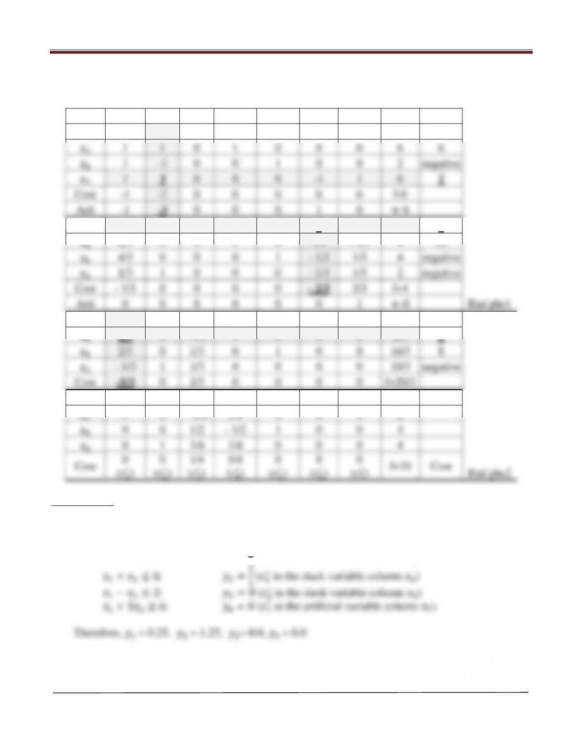
Standard LP form:
Chapter 8 Linear Programming Methods for Optimum Design
Table E8.55
Basic
1
2
3
4
5
6
7
b
ratio
3
-1
3
1
0
0
0
0
10
10/3
4
1
1
0
1
0
0
0
6
6
5
1
-1
0
0
1
0
0
2
negative
7
1
3
0
0
0
-1
1
6
2
Cost
-1
-2
0
0
0
0
0
f-0
Arti
-1
-3
0
0
0
1
0
w-6
3
-2
0
1
0
0
1
-1
4
4
4
2/3
0
0
1
0
1/3
– 1/3
4
12
5
4/3
0
0
0
1
– 1/3
1/3
4
negative
2
1/3
1
0
0
0
– 1/3
1/3
2
negative
Cost
– 1/3
0
0
0
0
– 2/3
2/3
f+4
Arti
0
0
0
0
0
0
1
w-0
End phs1
6
-2
0
1
0
0
1
-1
4
negative
4
4/3
0
– 1/3
1
0
0
0
8/3
2
5
2/3
0
1/3
0
1
0
0
16/3
8
2
– 1/3
1
1/3
0
0
0
0
10/3
negative
Cost
-5/3
0
2/3
0
0
0
0
f+20/3
6
0
0
1/2
3/2
0
1
-1
8
1
1
0
– 1/4
3/4
0
0
0
2
5
0
0
1/2
– 1/2
1
0
0
4
2
0
1
1/4
1/4
0
0
0
4
0
0
1/4
5/4
0
0
0
Chapter 8 Linear Programming Methods for Optimum Design
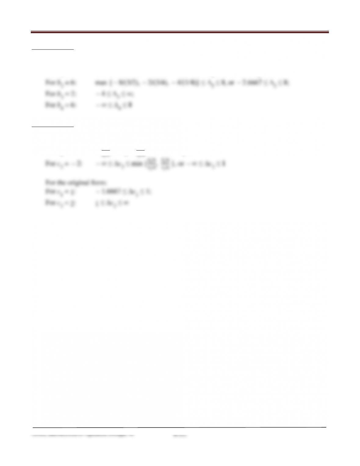
Exercise 8.110
Referring to Exercise 8.55 and the final tableau in Table E8.55, we can find the ranges for RHS by
Theorem 8.6 as follows:
For b1 = 10: max {
−
8/(1/2),
−
4/(1/2),
−
4/(1/4)} ≤ ∆1 ≤ 8, or
−
8 ≤ ∆1 ≤ 8;
−
−
−
−
−
−
Exercise 8.132
Referring to Exercise 8.55 and final tableau in Table E8.55, we can find the ranges for cost
coefficients by Theorem 8.8 as follows:
For c1 =
−
1:
−
1/4
−
1 ≤ ∆c1 ≤ 1.6667;
−
−
−
Arora, Introduction to Optimum Design, 4e
8-53
8.56 ________________________________________________________________________________
Solve the following LP problem by the Simplex method and verify the solution graphically,
whenever possible.
Maximize = 41+ 22
Subject to −21+2≤4
1+ 22≥2
1,2≥0
Solution:
Standard LP form:
Table E8.56
Basic
1
2
3
4
5
b
ratio
3
-2
1
1
0
0
4
4
5
1
2
0
-1
1
2
1
Cost
-4
-2
0
0
0
f-0
Arti
-1
-2
0
1
0
w-2
3
-2.5
0
1
0.5
-0.5
3
negative
2
0.5
1
0
-0.5
0.5
1
2
Cost
-3
0
0
-1
1
f+2
Arti
0
0
0
0
1
w-0
End phs1
3
0
5
1
-2
2
8
1
1
2
0
-1
1
2
Cost
0
6
0
-4
4
f+8
End phs2
Chapter 8 Linear Programming Methods for Optimum Design
8.57 ________________________________________________________________________________
Solve the following LP problem by the Simplex method and verify the solution graphically,
whenever possible.
Maximize =1+ 42
Subject to 1+ 22≤5
1+2= 4
1− 2≥3
1,2≥0
Solution:
Standard LP form:
Table E8.57
Basic
1
2
3
4
5
6
b
ratio
3
1
2
1
0
0
0
5
5
5
1
1
0
0
1
0
4
4
6
1
-1
0
-1
0
1
3
3
Cost
-1
-4
0
0
0
0
f-0
Arti
-2
0
0
1
0
0
w-7
3
0
3
1
1
0
-1
2
2/3
5
0
2
0
1
1
-1
1
1/2
1
1
-1
0
-1
0
1
3
negative
Cost
0
-5
0
-1
0
1
f+3
Arti
0
-2
0
-1
0
2
w-1
3
0
0
1
-0.5
-1.5
0.5
0.5
2
0
1
0
0.5
0.5
-0.5
0.5
1
1
0
0
-0.5
0.5
0.5
3.5
0
(1
′)
0
(2
′)
0
(3
′)
1.5
(4
′)
2.5
(5
-1.5
(6
′)
Arti
0
0
0
0
1
1
w-0
End phs1
End phs2
Exercise 8.90
From the final tableau for Exercise 8.57,
3 and 5 are slack variables; 4 is surplus variable; 6 is artificial variable.
′ in the slack variable column 3)
Exercise 8.112
Referring to Exercise 8.57 and the final tableau in Table E8.57, we can find the ranges for RHS by
Theorem 8.6 as follows:
0.5,−3.5
0.5 } ≤ ∆3 ≤0.5
0.5 or
Exercise 8.134
Referring to Exercise 8.57 and final tableau in Table E8.57, we can find the ranges for cost
coefficients by Theorem 8.8 as follows:
0.5 or
For the original form:
Arti
0
0
0
0
1
1
w-0
8.58 ________________________________________________________________________________
Solve the following LP problem by the Simplex method and verify the solution graphically,
whenever possible.
Maximize =1+ 42
Subject to 1+ 22≤5
21+2= 4
1− 2≥1
1,2≥0
Solution:
Standard LP form:
Table E8.58
Basic
1
2
3
4
5
6
b
ratio
3
1
2
1
0
0
0
5
5
5
2
1
0
0
1
0
4
2
6
1
-1
0
-1
0
1
1
1
Cost
-1
-4
0
0
0
0
f-0
Arti
-3
0
0
1
0
0
w-5
3
0
3
1
1
0
-1
4
4/3
5
0
3
0
2
1
-2
2
2/3
1
1
-1
0
-1
0
1
1
-1
Cost
0
-5
0
-1
0
1
f+1
Arti
0
-3
0
-2
0
3
w-2
3
0
0
1
-1
-1
1
2
2
0
1
0
2/3
1/3
– 2/3
0.666667
1
1
0
0
– 1/3
1/3
1/3
1.666667
0
0
0
7/3
5/3
-7/3
Chapter 8 Linear Programming Methods for Optimum Design
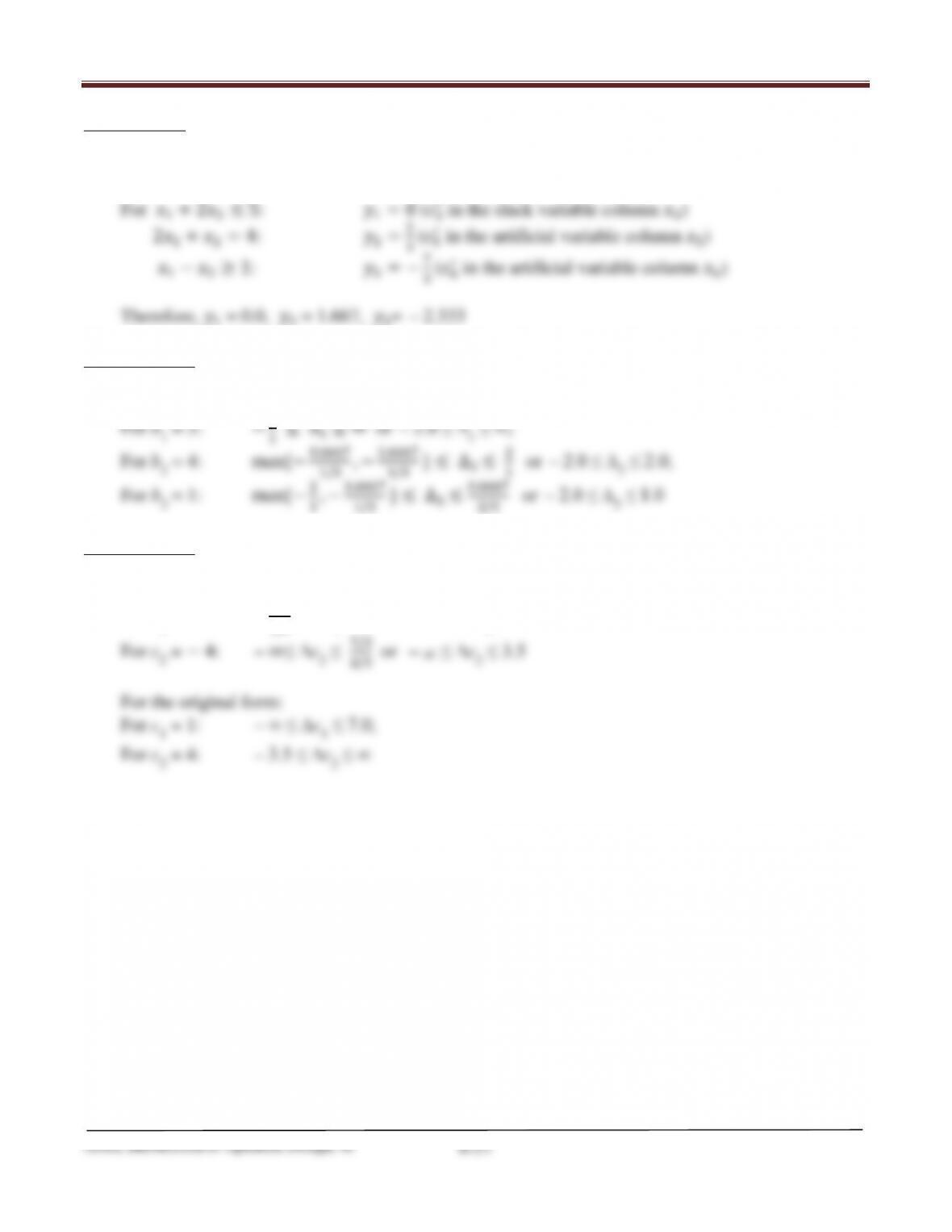
Exercise 8.91
From the final tableau for Exercise 8.58,
3 is slack variable; 4 is surplus variable; 5 and 6 are artificial variables.
′ in the slack variable column 3)
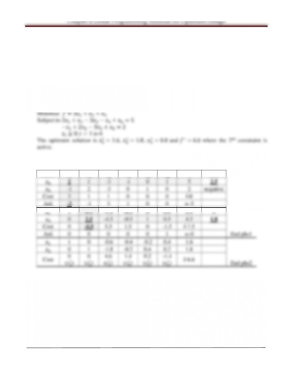
Exercise 8.113
Referring to Exercise 8.58 and the final tableau in Table E8.58, we can find the ranges for RHS by
Theorem 8.6 as follows:
−
−
1,−1.6667
1/3 } ≤ ∆3 ≤0.6667
2/3 or
Exercise 8.135
Referring to Exercise 8.58 and final tableau in Table E8.58, we can find the ranges for cost
coefficients by Theorem 8.8 as follows:
For c1 = − 1:
−
7/3
1/3 ≤ ∆c1 ≤ ∞ or
−
7.0 ≤ ∆c1 ≤ ∞;
−
Arora, Introduction to Optimum Design, 4e
8-58
8.59 ________________________________________________________________________________
Solve the following LP problem by the Simplex method and verify the solution graphically,
whenever possible.
Minimize = 31+2+3
Subject to −21− 2+ 33≤ −5
1−22+ 33≥ −2
1,2,3≥0
Solution:
Standard LP form:
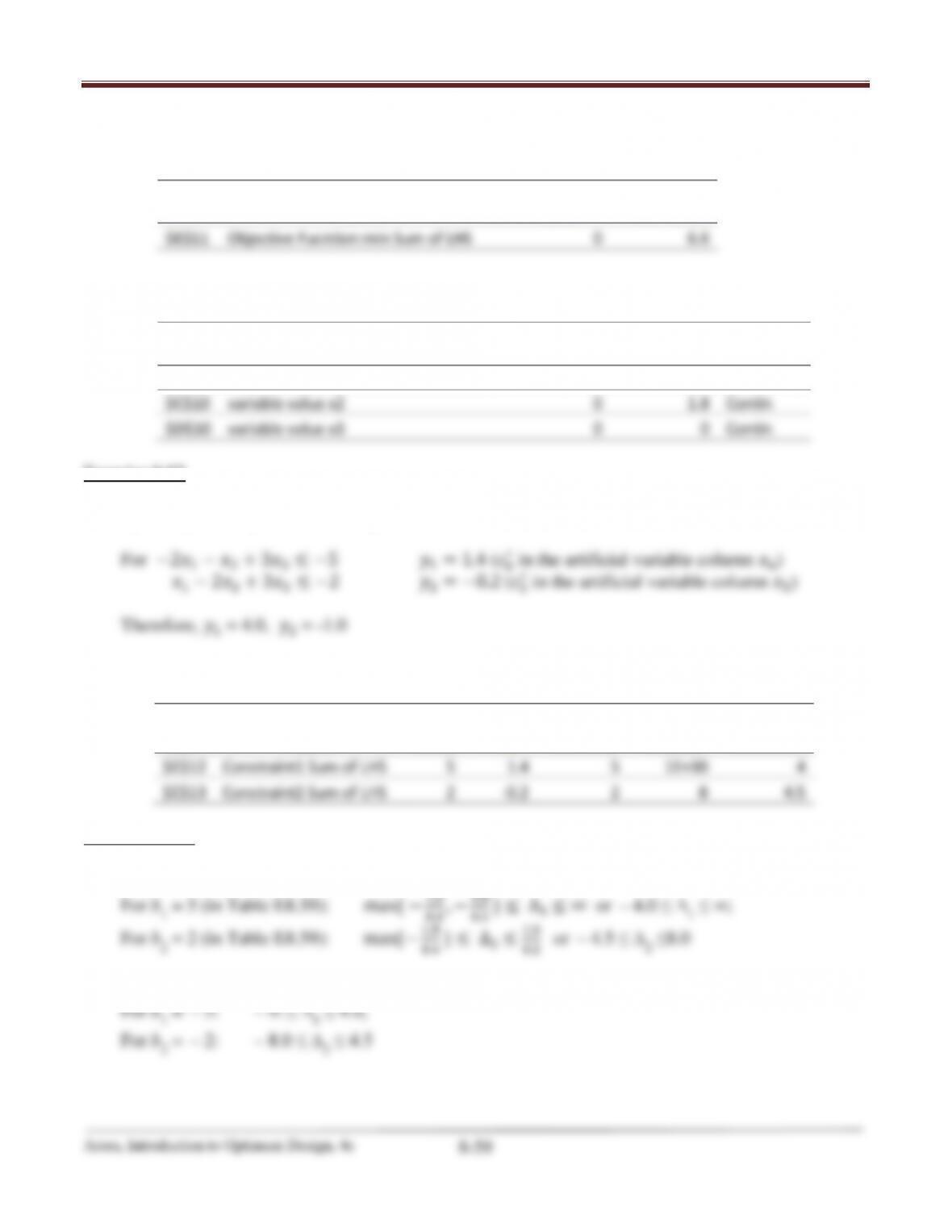
Table E8.59A
Basic
1
2
3
4
5
6
b
ratio
6
2
1
-3
-1
0
1
5
2.5
5
-1
2
-3
0
1
0
2
negative
Cost
3
1
1
0
0
0
f-0
Arti
-2
-1
3
1
0
0
w-5
1
1
0.5
-1.5
-0.5
0
0.5
2.5
5
5
0
2.5
-4.5
-0.5
1
0.5
4.5
1.8
Cost
0
-0.5
5.5
1.5
0
-1.5
f-7.5
Arti
0
0
0
0
0
1
w-0
End phs1
1
1
0
-0.6
-0.4
-0.2
0.4
1.6
2
0
1
-1.8
-0.2
0.4
0.2
1.8
End phs2
0
0
4.6
1.4
0.2
-1.4
Chapter 8 Linear Programming Methods for Optimum Design
Table E8.59B LP Solver
Objective Cell (Min)
Cell
Name
Original
Value
Final Value
$E$11
Objective Fucntion:min Sum of LHS
0
6.6
Variable Cells
Cell
Name
Original
Value
Final Value
Integer
$B$10
variable value x1
0
1.6
Contin
$C$10
variable value x2
0
1.8
Contin
$D$10
variable value x3
0
0
Contin
Exercise 8.92
From the final tableau for Exercise 8.59,
4 and 5 are surplus variables; 6 and 7 are artificial variables.
Table 8.92 LP Solver
Constraints
Final
Shadow
Constraint
Allowable
Allowable
Cell
Name
Value
Price
R.H. Side
Increase
Decrease
$E$12
Constraint1 Sum of LHS
5
1.4
5
1E+30
4
$E$13
Constraint2 Sum of LHS
2
–0.2
2
8
4.5
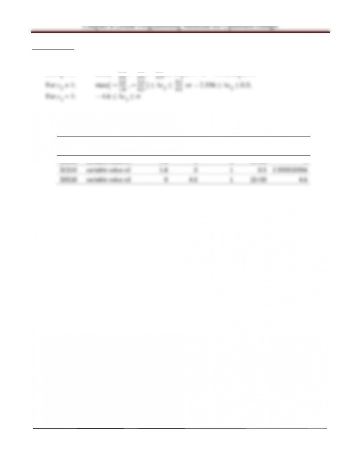
Exercise 8.114
Referring to Exercise 8.59 and the final tableau in Table E8.59, we can find the ranges for RHS by
Theorem 8.6 as follows:
0.4 } ≤ ∆2 ≤1.6
0.2 or
Therefore,
Arora, Introduction to Optimum Design, 4e
8-60
Exercise 8.136
Referring to Exercise 8.59 and final tableau in Table E8.59, we can find the ranges for cost
coefficients by Theorem 8.8 as follows:
For c1 = 3: max { −4.6
−
1.0 ≤ ∆c1 ≤ ∞;
−
−
Table 8.136 LP Solver
Variable Cells
Final
Reduced
Objective
Allowable
Allowable
Cell
Name
Value
Cost
Coefficient
Increase
Decrease
$B$10
variable value x1
1.6
0
3
1E+30
1
$C$10
variable value x2
1.8
0
1
0.5
2.555555556
$D$10
variable value x3
0
4.6
1
1E+30
4.6