Chapter 8 Linear Programming Methods for Optimum Design
[x1,x2]=meshgrid(–1:0.05:10, –1:0.05:10);
f=–4*x1–5*x2;
g1=x1–2*x2+10;
g2=3*x1+2*x2–18;
cv3=[0:0.1:1.8];
contour(x1,x2,g2,cv3,‘g’);
cv4=[0:0.01:0.02];
contour(x1,x2,g2,cv4,‘k’);
cv5=[0:0.05:0.5];
Chapter 8 Linear Programming Methods for Optimum Design
Arora, Introduction to Optimum Design, 4e
8-102
8.77 ________________________________________________________________________________
Solve the following LP problem by the Simplex method and verify the solution graphically,
whenever possible.
Referring to Exercise 2.2, we have:
Maximize =48+28
Subject to 0.6+ 0.8 ≤ 20,000
0.4+ 0.2 ≤ 10,000
≤ 20,000
≤ 30,000
, ≥ 0
Solution:
Standard LP form:
Chapter 8 Linear Programming Methods for Optimum Design
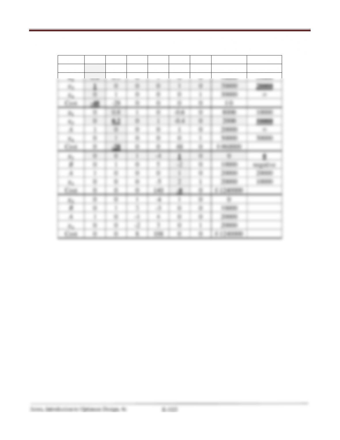
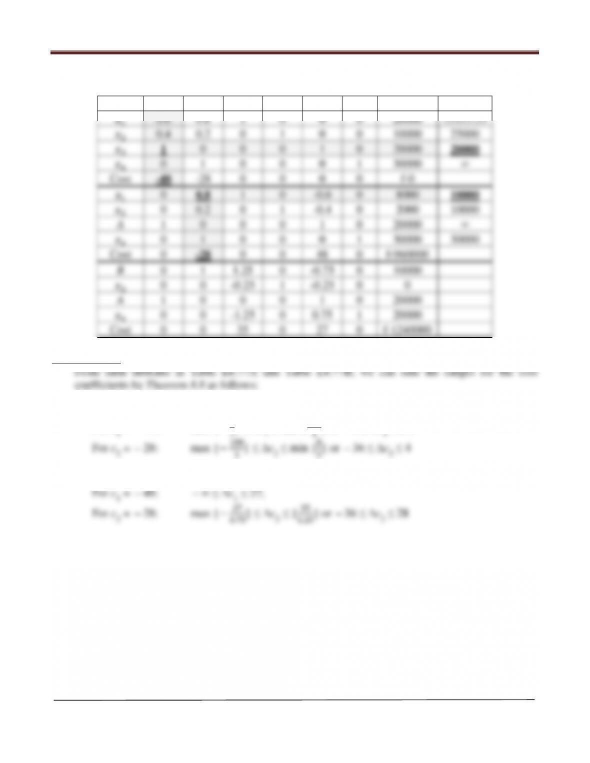
Table E8.77A
Basic
A
B
1
2
3
4
b
ratio
1
0.6
0.8
1
0
0
0
20000
33333.33
2
0.4
0.2
0
1
0
0
10000
25000
3
1
0
0
0
1
0
20000
20000
4
0
1
0
0
0
1
30000
∞
Cost
-48
-28
0
0
0
0
f-0
1
0
0.8
1
0
-0.6
0
8000
10000
2
0
0.2
0
1
-0.4
0
2000
10000
A
1
0
0
0
1
0
20000
∞
4
0
1
0
0
0
1
30000
30000
Cost
0
-28
0
0
48
0
f-960000
1
0
0
1
-4
1
0
0
0
B
0
1
0
5
-2
0
10000
negative
A
1
0
0
0
1
0
20000
20000
4
0
0
0
-5
2
1
20000
10000
Cost
0
0
0
140
-8
0
f-1240000
3
0
0
1
-4
1
0
0
B
0
1
2
-3
0
0
10000
A
1
0
-1
4
0
0
20000
4
0
0
-2
3
0
1
20000
Cost
0
0
8
108
0
0
f-1240000
Chapter 8 Linear Programming Methods for Optimum Design
Arora, Introduction to Optimum Design, 4e
8-104
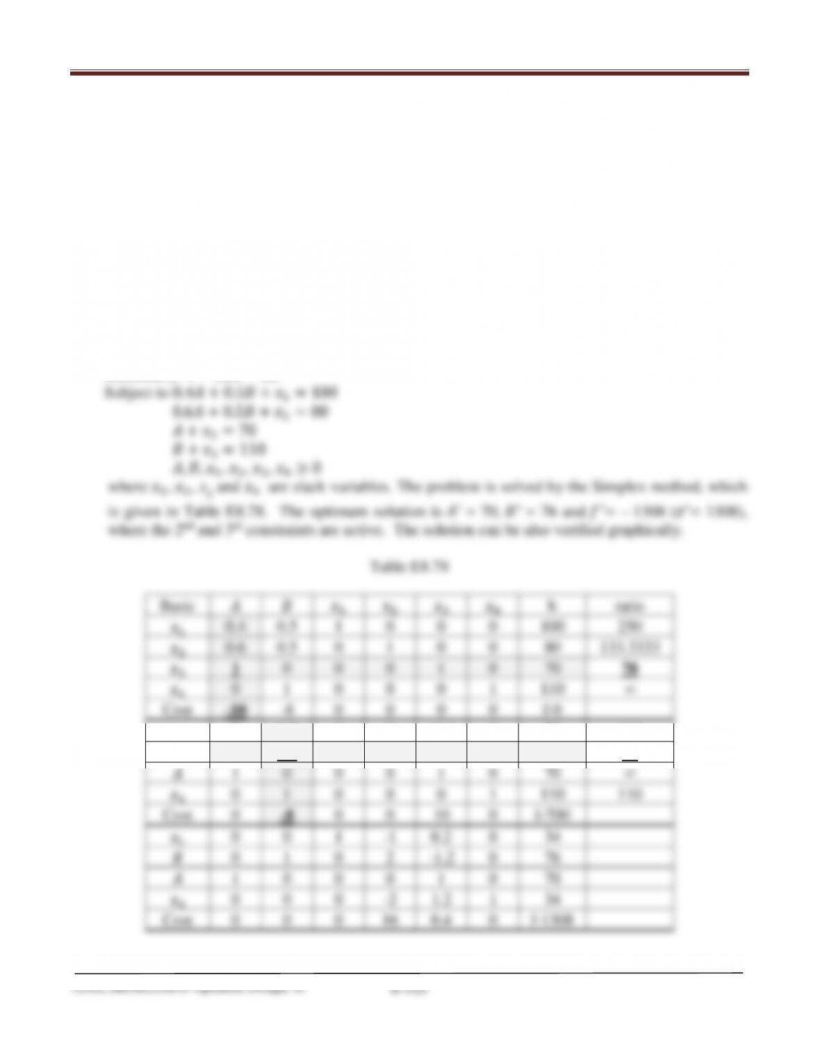
Table E8.77B
Basic
A
B
1
2
3
4
b
ratio
1
0.6
0.8
1
0
0
0
20000
33333.33
2
0.4
0.2
0
1
0
0
10000
25000
3
1
0
0
0
1
0
20000
20000
4
0
1
0
0
0
1
30000
∞
Cost
-48
-28
0
0
0
0
f-0
1
0
0.8
1
0
-0.6
0
8000
10000
2
0
0.2
0
1
-0.4
0
2000
10000
A
1
0
0
0
1
0
20000
∞
4
0
1
0
0
0
1
30000
30000
Cost
0
-28
0
0
48
0
f-960000
B
0
1
1.25
0
-0.75
0
10000
2
0
0
-0.25
1
-0.25
0
0
A
1
0
0
0
1
0
20000
4
0
0
-1.25
0
0.75
1
20000
Cost
0
0
35
0
27
0
f-1240000
Exercise 8.154
1. Use final tableau in Table E8.77A.
For c1 =
−
48: max {−8
−
8 ≤ ∆c1 ≤ 27;
−
−
2. Use final tableau in Table E8.77B.
Chapter 8 Linear Programming Methods for Optimum Design
8.78 ________________________________________________________________________________
Solve the following LP problem by the Simplex method and verify the solution graphically,
whenever possible.
Referring to Exercise 2.6, we have:
Maximize =10+ 8
Subject to 0.4+ 0.5 ≤ 100
0.6+ 0.5 ≤ 80
≤ 70
≤ 110
, ≥ 0
Solution:
Standard LP form:
Minimize =−10 − 8
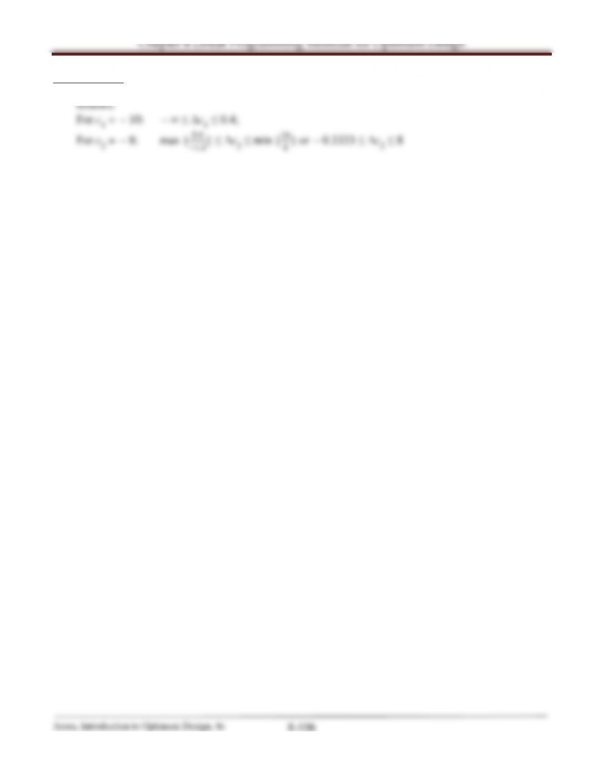
Exercise 8.155
From the final tableau in Table E8.78, we can find the ranges for cost coefficients by Theorem 8.8 as
Chapter 8 Linear Programming Methods for Optimum Design
8.79 ________________________________________________________________________________
Solve the following LP problem by the Simplex method and verify the solution graphically,
whenever possible.
Referring to Exercise 2.7, we have
Minimize = 2+
Subject to + 2 ≥ 5
3+ 2 ≥ 4
, ≥ 0
Solution:
Standard LP form:
Minimize = 2+
Table E8.79
Basic
1
2
3
4
b
ratio
3
1
2
-1
0
1
0
5
2.5
4
3
2
0
-1
0
1
4
2
Cost
2
1
0
0
0
0
f-0
Arti
-4
-4
1
1
0
0
w-9
3
-2
0
-1
1
1
-1
1
1
1.5
1
0
-0.5
0
0.5
2
negative
Cost
0.5
0
0
0.5
0
-0.5
f-2
Arti
2
0
1
-1
0
2
w-1
2
-2
0
-1
1
1
-1
1
0.5
1
-0.5
0
0.5
0
2.5
Cost
1.5
0
0.5
0
-0.5
0
f-2.5
Arti
0
0
0
0
1
1
w-0
End phs1
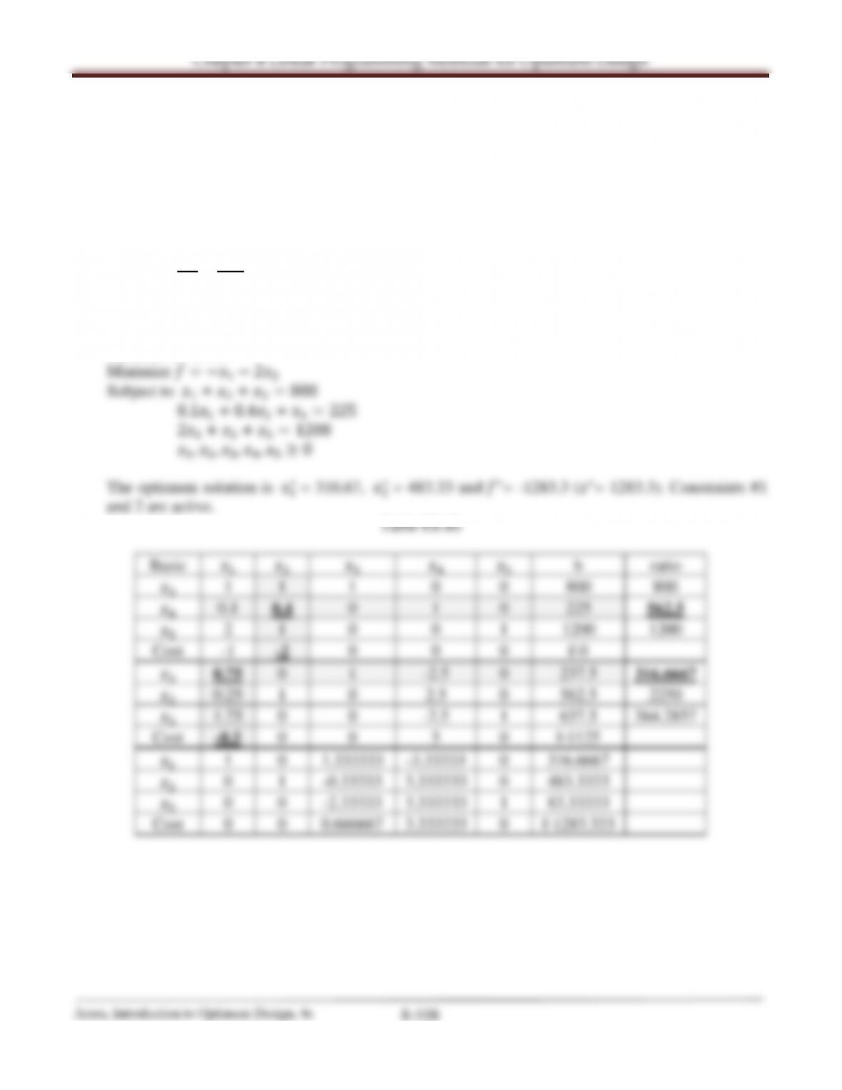
8.80 ________________________________________________________________________________
Solve the following LP problem by the Simplex method and verify the solution graphically,
whenever possible.
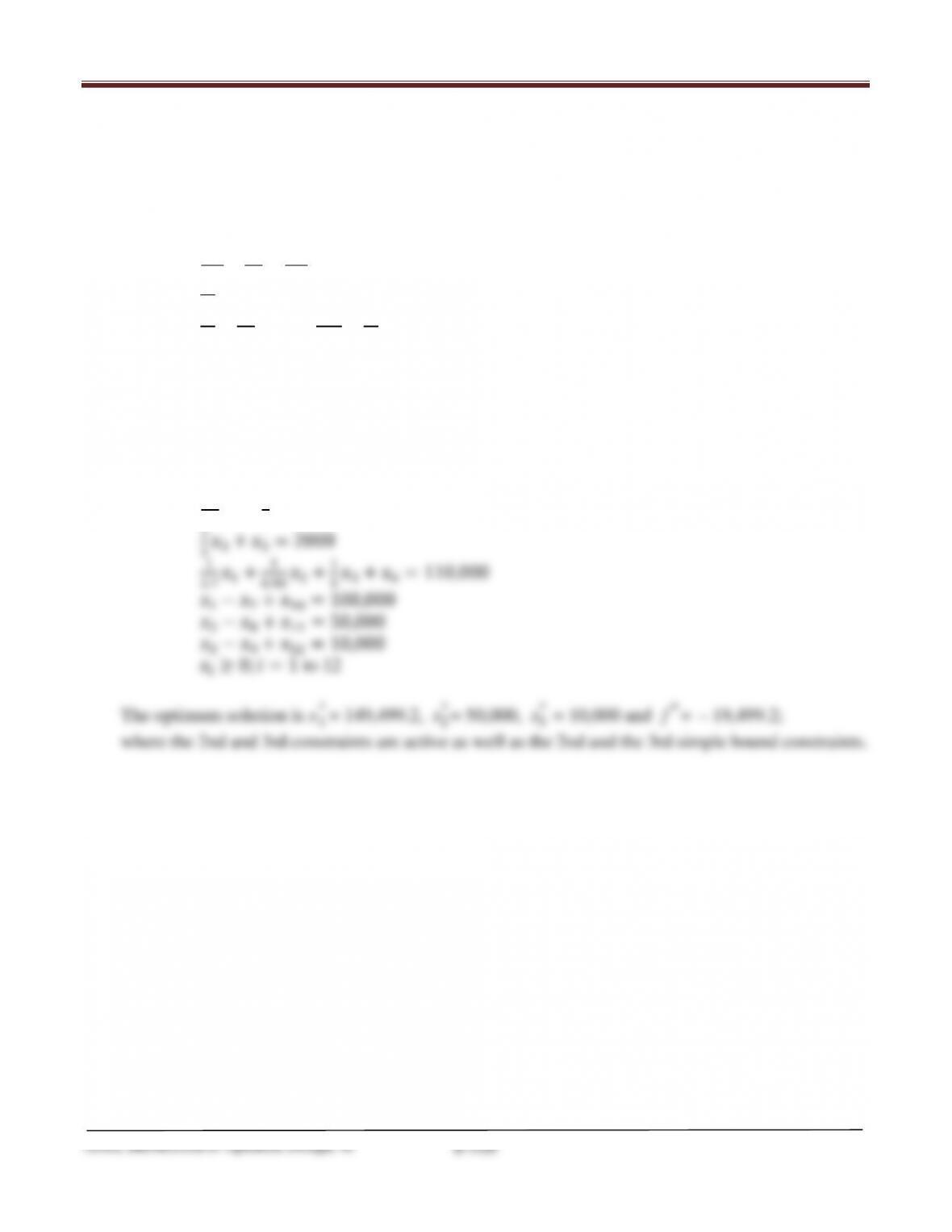
Referring to Exercise 2.8, we have:
Maximize =1+ 22
Subject to 1+2≤800
0.11+ 0.42≤225
1
600 +2
1200 ≤1
1,2≥0
Solution:
Standard LP form:
Chapter 8 Linear Programming Methods for Optimum Design
8.81 ________________________________________________________________________________
Solve the following LP problem by the Simplex method and verify the solution graphically,
whenever possible.
Referring to Exercise 2.18, we have:
Maximize = 0.11+ 0.082+ 0.053
Subject to 21
3×1
0.9+33
5≤250,000
3
5≤2000
1
3×1
0.9+2×1
0.95 +3
5≤110,000
1≥100,000
2≥50,000
3≥10,000
Solution:
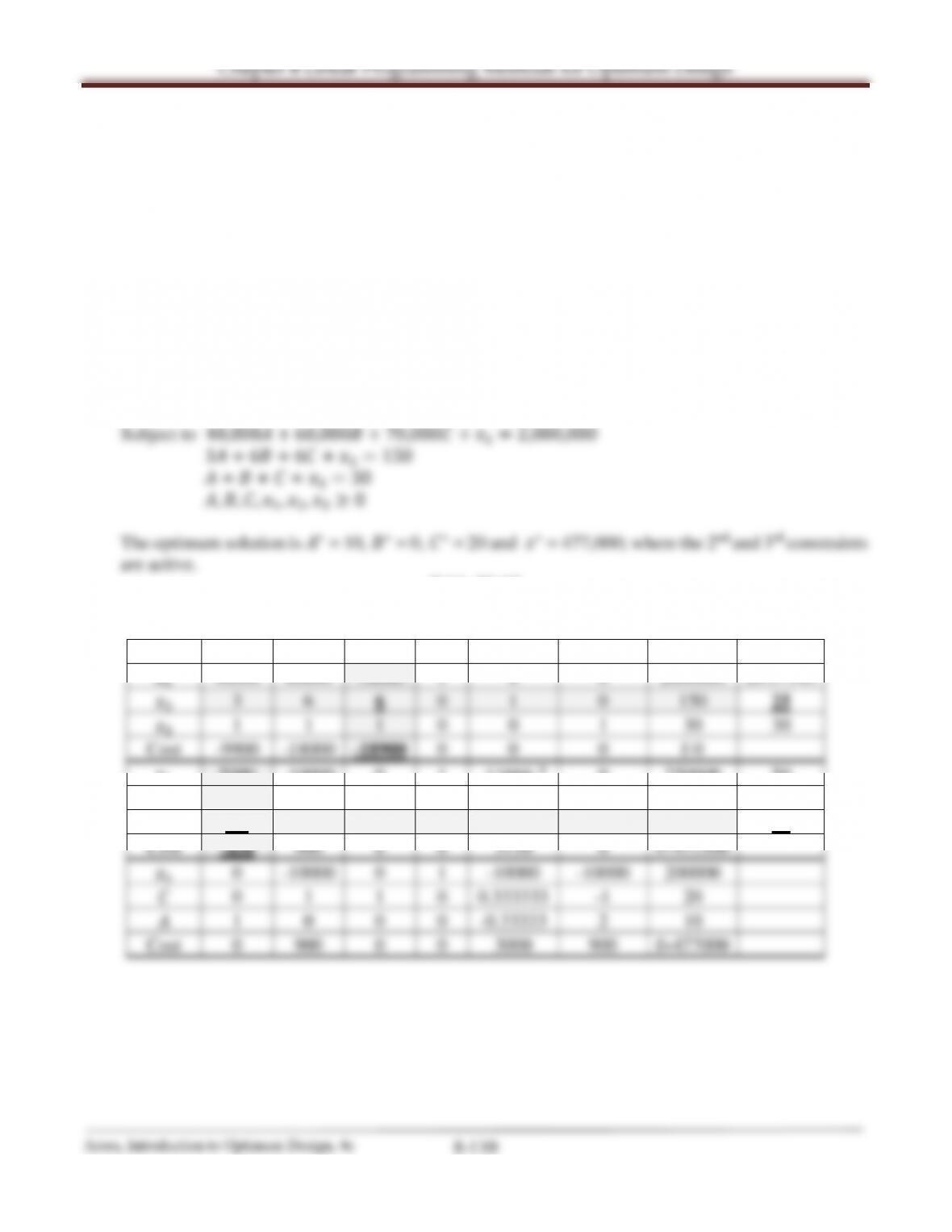
Standard LP form:
Minimize =−0.11−0.082−0.053
Subject to 2
2.71+3
53+4=250,000
8.82 ________________________________________________________________________________
Solve the following LP problem by the Simplex method and verify the solution graphically,
whenever possible.
Referring to Exercise 2.20, we have:
Maximize =9900+18000+18900
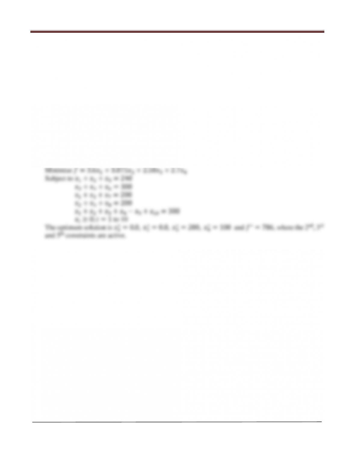
Subject to 40,000+60,000+70,000 ≤ 2,000,000
3+ 6+ 6 ≤ 150
++ ≤ 30
,, ≥ 0
Solution:
Standard LP form:
Minimize =−9900 − 18000 − 18900
Table E8.82
Basic
1
2
3
b
ratio
1
40000
60000
70000
1
0
0
2000000
28.57143
2
3
6
6
0
1
0
150
25
3
1
1
1
0
0
1
30
30
Cost
-9900
-18000
-18900
0
0
0
f-0
1
5000
-10000
0
1
-11666.7
0
250000
50
0.5
1
1
0
0.166667
0
25
50
3
0.5
0
0
0
-0.16667
1
5
10
Cost
-450
900
0
0
3150
0
f+472500
1
0
-10000
0
1
-10000
-10000
200000
0
1
1
0
0.333333
-1
20
1
0
0
0
-0.33333
2
10
Cost
0
900
0
0
3000
900
f+477000
Chapter 8 Linear Programming Methods for Optimum Design
Arora, Introduction to Optimum Design, 4e
8-111
8.83 ________________________________________________________________________________
Solve the following LP problem by the Simplex method and verify the solution graphically,
whenever possible.
Referring to Section 2.4, we have:
Minimize = 3.61+ 3.0752+ 2.583+ 2.74
Subject to 1+2≤240
3+4≤300
1+3≤200
2+4≤200
1+2+3+4≥300
≥0; = 1 to 4
Solution:
Standard LP form:
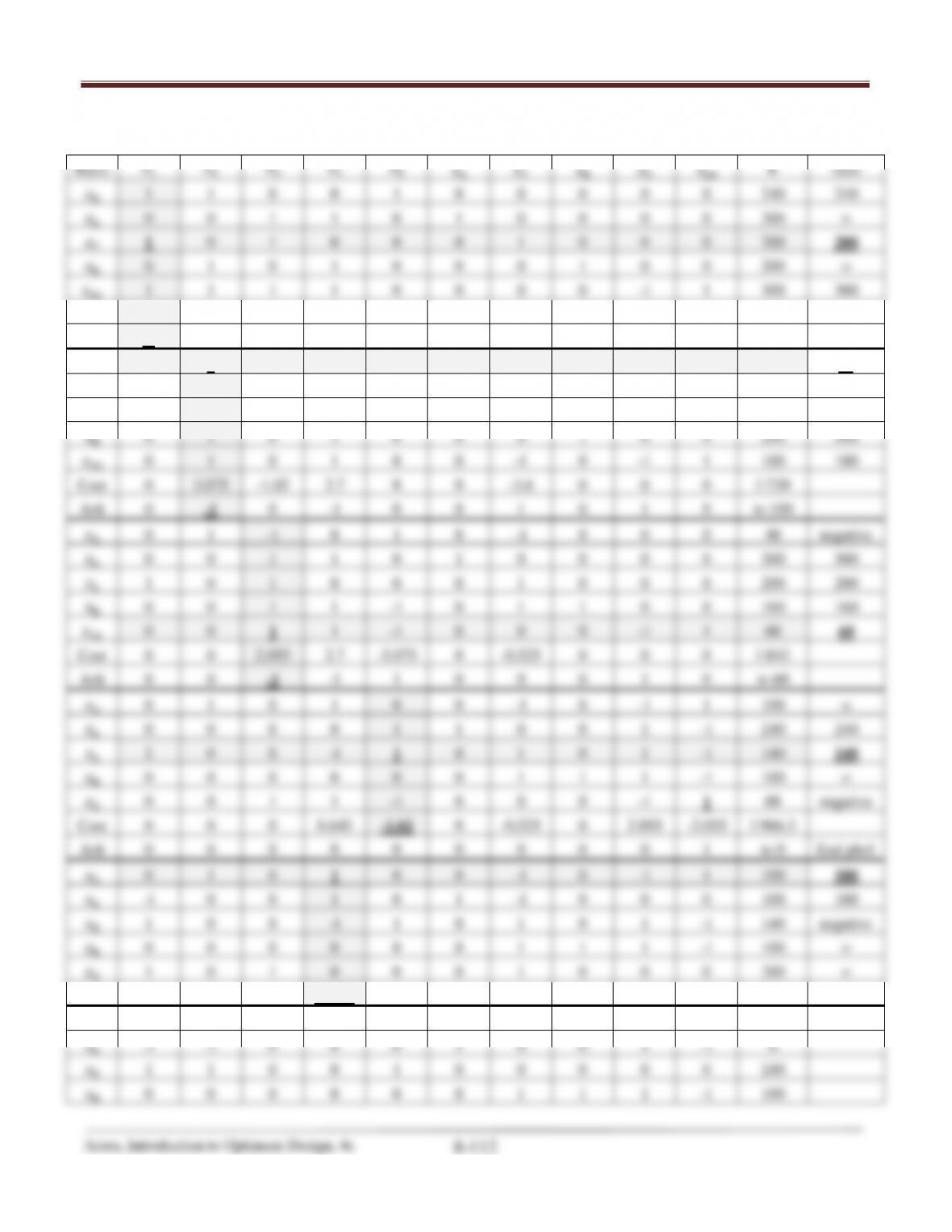
Chapter 8 Linear Programming Methods for Optimum Design
Table E8.83
Basic
1
2
3
4
5
6
7
8
9
10
b
ratio
5
1
1
0
0
1
0
0
0
0
0
240
240
6
0
0
1
1
0
1
0
0
0
0
300
∞
7
1
0
1
0
0
0
1
0
0
0
200
200
8
0
1
0
1
0
0
0
1
0
0
200
∞
10
1
1
1
1
0
0
0
0
-1
1
300
300
Cost
3.6
3.075
2.58
2.7
0
0
0
0
0
0
f-0
Arti
-1
-1
-1
-1
0
0
0
0
1
0
w-300
5
0
1
-1
0
1
0
-1
0
0
0
40
40
6
0
0
1
1
0
1
0
0
0
0
300
∞
1
1
0
1
0
0
0
1
0
0
0
200
∞
8
0
1
0
1
0
0
0
1
0
0
200
200
10
0
1
0
1
0
0
-1
0
-1
1
100
100
Cost
0
3.075
–1.02
2.7
0
0
–3.6
0
0
0
f-720
Arti
0
-1
0
-1
0
0
1
0
1
0
w-100
2
0
1
-1
0
1
0
-1
0
0
0
40
negative
6
0
0
1
1
0
1
0
0
0
0
300
300
1
1
0
1
0
0
0
1
0
0
0
200
200
8
0
0
1
1
-1
0
1
1
0
0
160
160
10
0
0
1
1
-1
0
0
0
-1
1
60
60
Cost
0
0
2.055
2.7
–3.075
0
–0.525
0
0
0
f-843
Arti
0
0
-1
-1
1
0
0
0
1
0
w-60
2
0
1
0
1
0
0
-1
0
-1
1
100
∞
6
0
0
0
0
1
1
0
0
1
-1
240
240
1
1
0
0
-1
1
0
1
0
1
-1
140
140
8
0
0
0
0
0
0
1
1
1
-1
100
∞
3
0
0
1
1
-1
0
0
0
-1
1
60
negative
Cost
0
0
0
0.645
–1.02
0
–0.525
0
2.055
–2.055
f-966.3
Arti
0
0
0
0
0
0
0
0
0
1
w-0
End phs1
2
0
1
0
1
0
0
-1
0
-1
1
100
100
6
-1
0
0
1
0
1
-1
0
0
0
100
100
5
1
0
0
-1
1
0
1
0
1
-1
140
negative
8
0
0
0
0
0
0
1
1
1
-1
100
∞
3
1
0
1
0
0
0
1
0
0
0
200
∞
Cost
1.02
0
0
–0.375
0
0
0.495
0
3.075
–3.075
f-823.5
4
0
1
0
1
0
0
-1
0
-1
1
100
6
-1
-1
0
0
0
1
0
0
1
-1
0
5
1
1
0
0
1
0
0
0
0
0
240
8
0
0
0
0
0
0
1
1
1
-1
100