CHAPTER
6
Optimum Design: Numerical Solution Process and
Excel Solver
Section 6.5 Excel Solver for Unconstrained Optimization Problems
6.1_________________________________________________________________________________
Solve the following problem using Excel Solver (choose any reasonable starting point):
Exercise 4.32
The annual operating cost U for an electrical line system is given by the following expression
=(21.9+07)
2+(3.9+06)+(1.0+03)
where V=line voltage in kilovolts and C=line conductance in ohms. Find stationary points for the
function, and determine V and C to minimize the operating cost.
Solution
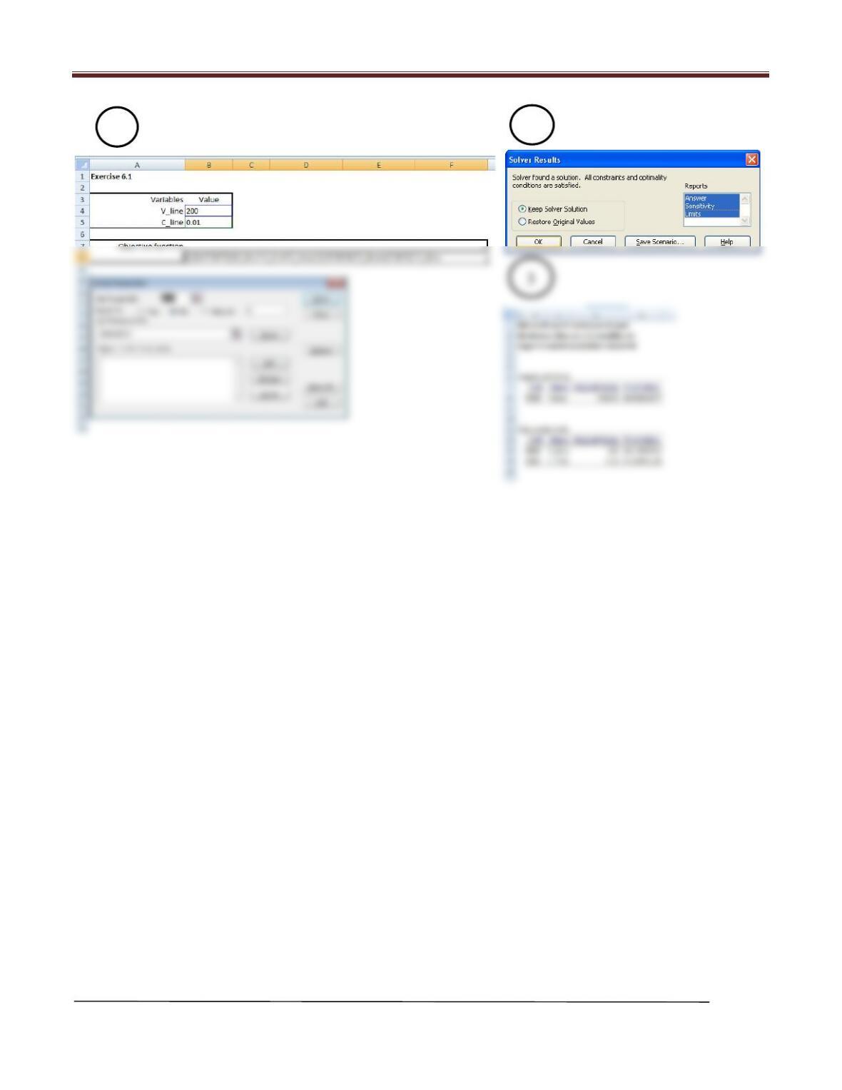
(1) One possible format for setting up the Excel worksheet for this problem is shown below.
Variables V and C have been renamed V_line and C_line respectively. The objective
(3) The answer report shows that for initial design variable values of V_line=200 and C_line=0.01, a
Chapter 6 Optimum Design: Numerical Solution Process and Excel Solver
Arora, Introduction to Optimum Design, 4e
6-2
2
1
3
Chapter 6 Optimum Design: Numerical Solution Process and Excel Solver
Arora, Introduction to Optimum Design, 4e
6-3
6.2________________________________________________________________________________
Solve the following problem using Excel Solver (choose any reasonable starting point):
Exercise 4.39
(1,2)= 81
2+ 82
2−80�1
2+2
2−202+100 −80�1
2+2
2+202+ 100 −51−52
Solution
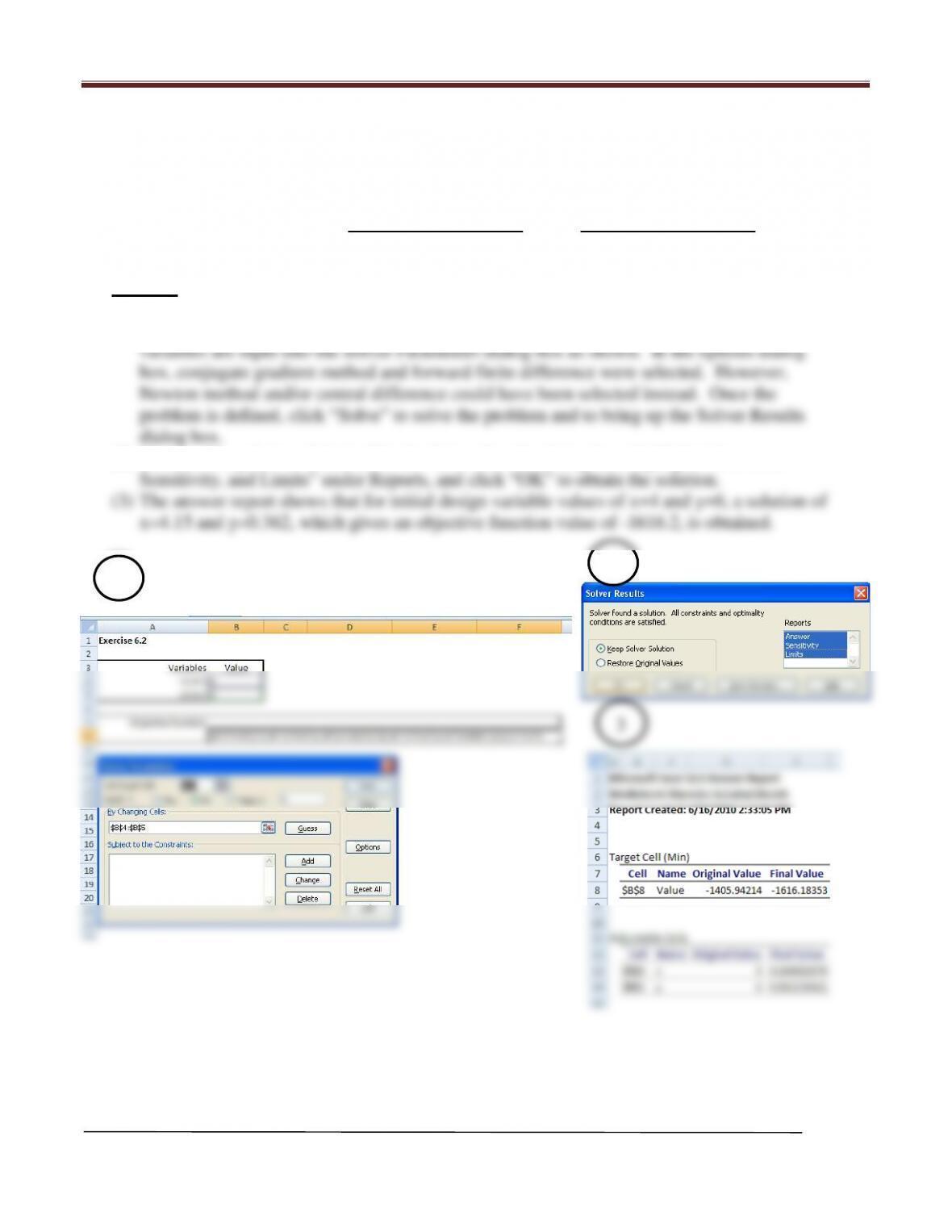
(1) One possible format for setting up the Excel worksheet for this problem is shown below.
Variables x1 and x2 have been renamed x and y respectively. The objective function and
(2) Choose “Keep Solver Solution” in the Solver Results dialog box, highlight “Answers,
1
2
Chapter 6 Optimum Design: Numerical Solution Process and Excel Solver
Arora, Introduction to Optimum Design, 4e
6-4
6.3_________________________________________________________________________________
Solve the following problem using Excel Solver (choose any reasonable starting point):
Exercise 4.40
(1,2)= 91
2+ 92
2−100�1
2+2
2−202+100 −64�1
2+2
2+162+64 −51−412
Solution
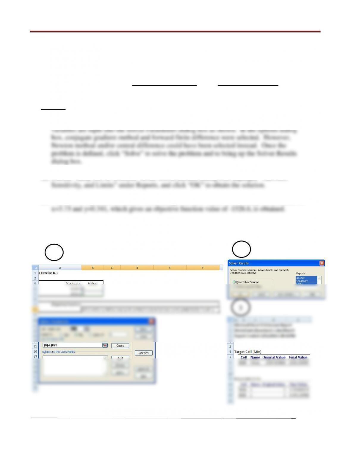
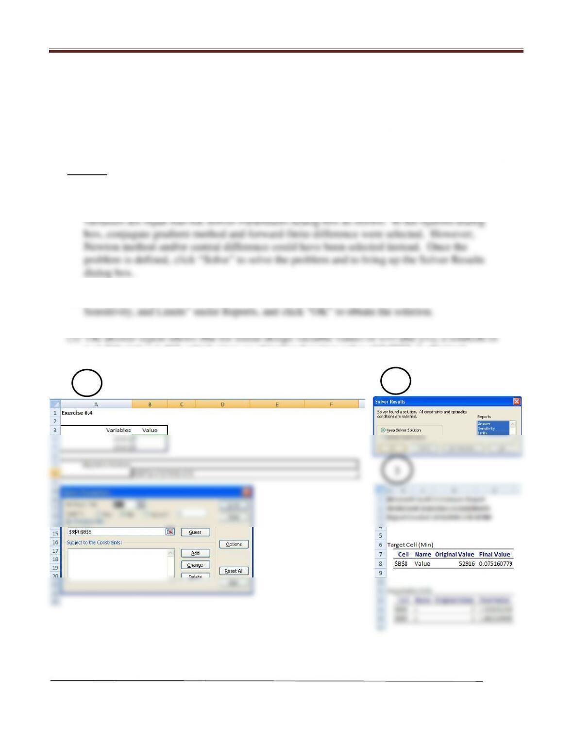
(1) One possible format for setting up the Excel worksheet for this problem is shown below.
Variables x1 and x2 have been renamed x and y respectively. The objective function and
(2) Choose “Keep Solver Solution” in the Solver Results dialog box, highlight “Answers,
(3) The answer report shows that for initial design variable values of x=5 and y=2, a solution of
3
1
2
Chapter 6 Optimum Design: Numerical Solution Process and Excel Solver
Arora, Introduction to Optimum Design, 4e
6-5
6.4 _________________________________________________________________________________
Solve the following problem using Excel Solver (choose any reasonable starting point):
Exercise 4.41
(1,2)=100(2− 1
2)2+ (1 − 1)2
Solution
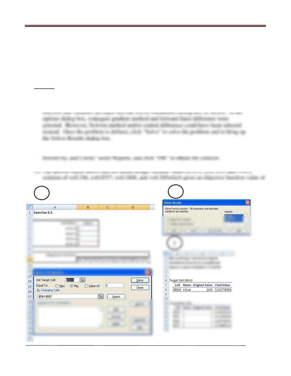
(1) One possible format for setting up the Excel worksheet for this problem is shown below.
Variables x1 and x2 have been renamed x and y respectively. The objective function and
(2) Choose “Keep Solver Solution” in the Solver Results dialog box, highlight “Answers,
x=1.216 and y=1.462, which gives an objective function value of 0.0752, is obtained.
3
1
2
Chapter 6 Optimum Design: Numerical Solution Process and Excel Solver
Arora, Introduction to Optimum Design, 4e
6-6
6.5 _________________________________________________________________________________
Solve the following problem using Excel Solver (choose any reasonable starting point):
Exercise 4.42
(1,2,3,4)=(1−102)2+ 5(3− 4)2+(2−23)4+10(1− 4)4
Solution
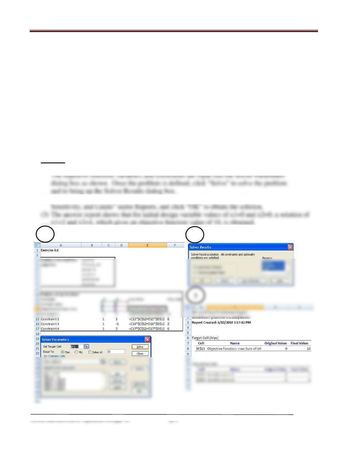
(1) One possible format for setting up the Excel worksheet for this problem is shown below.
Variables x1, x2, x3, and x4 have been renamed x, y, z, and v respectively. The objective
(2) Choose “Keep Solver Solution” in the Solver Results dialog box, highlight “Answers,
0.01578, is obtained.
3
2
1
Chapter 6 Optimum Design: Numerical Solution Process and Excel Solver
Section 6.6 Excel Solver for Linear Programming Problems
Solve the following LP problems using Excel Solver:
6.6 _________________________________________________________________________________
Solve the following LP problem using the Excel Solver:
Maximize z = x1 + 2x2
subject to −x1 + 3x2 ≤ 10
x1 + x2 ≤ 6
x1 − x2 ≤ 2
x1 + 3x2 ≥ 6
x1, x2 ≥ 0
Solution
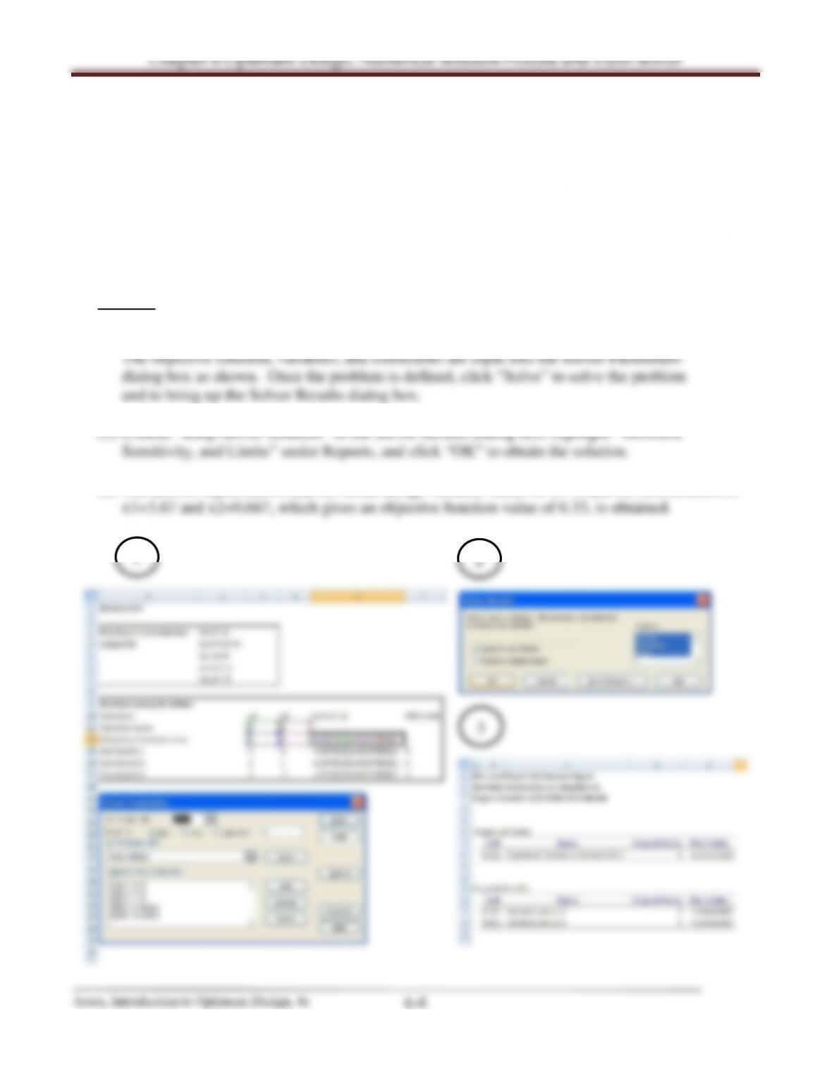
(1) One possible format for setting up the Excel worksheet for this problem is shown below.
(2) Choose “Keep Solver Solution” in the Solver Results dialog box, highlight “Answers,
1
2
3
Chapter 6 Optimum Design: Numerical Solution Process and Excel Solver
Arora, Introduction to Optimum Design, 4e
6-9
6.8 _________________________________________________________________________________
Solve the following LP problem using the Excel Solver:
Minimize f = 5x1 + 4x2 − x3
subject to x1 + 2x2 − x3 ≥ 1
2x1 + x2 + x3 ≥ 4
x1, x2 ≥ 0; x3 is unrestricted in sign
Solution
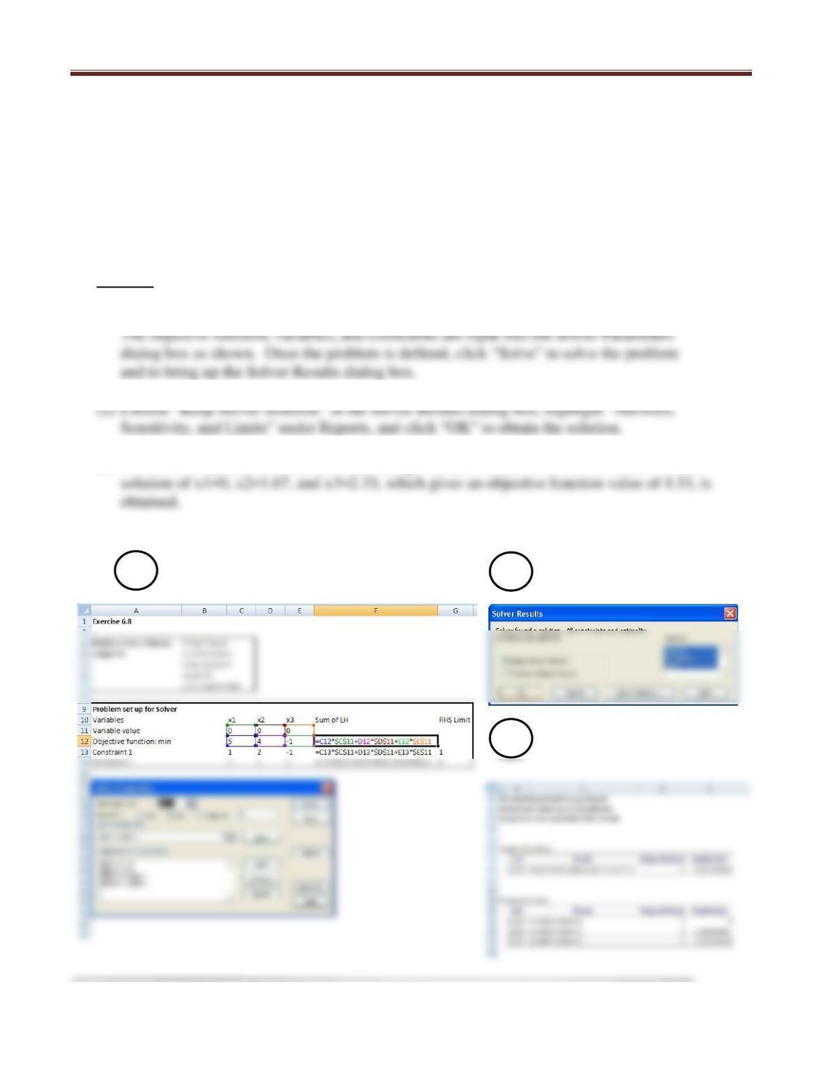
(1) One possible format for setting up the Excel worksheet for this problem is shown below.
(3) The answer report shows that for initial design variable values of x1=0, x2=0, and x3=0, a
1
2
3
Chapter 6 Optimum Design: Numerical Solution Process and Excel Solver
6.9 _________________________________________________________________________________
Solve the following LP problem using the Excel Solver:
Maximize z = 2x1 + 5x2 − 4.5x3 + 1.5x4
subject to 5x1 + 3x2 + 1.5x3 ≤ 8
1.8x1 − 6x2 + 4x3 + x4 ≥ 3
−3.6x1 + 8.2x2 + 7.5x3 + 5x4 = 15
xi ≥ 0; i = 1 to 4
Solution
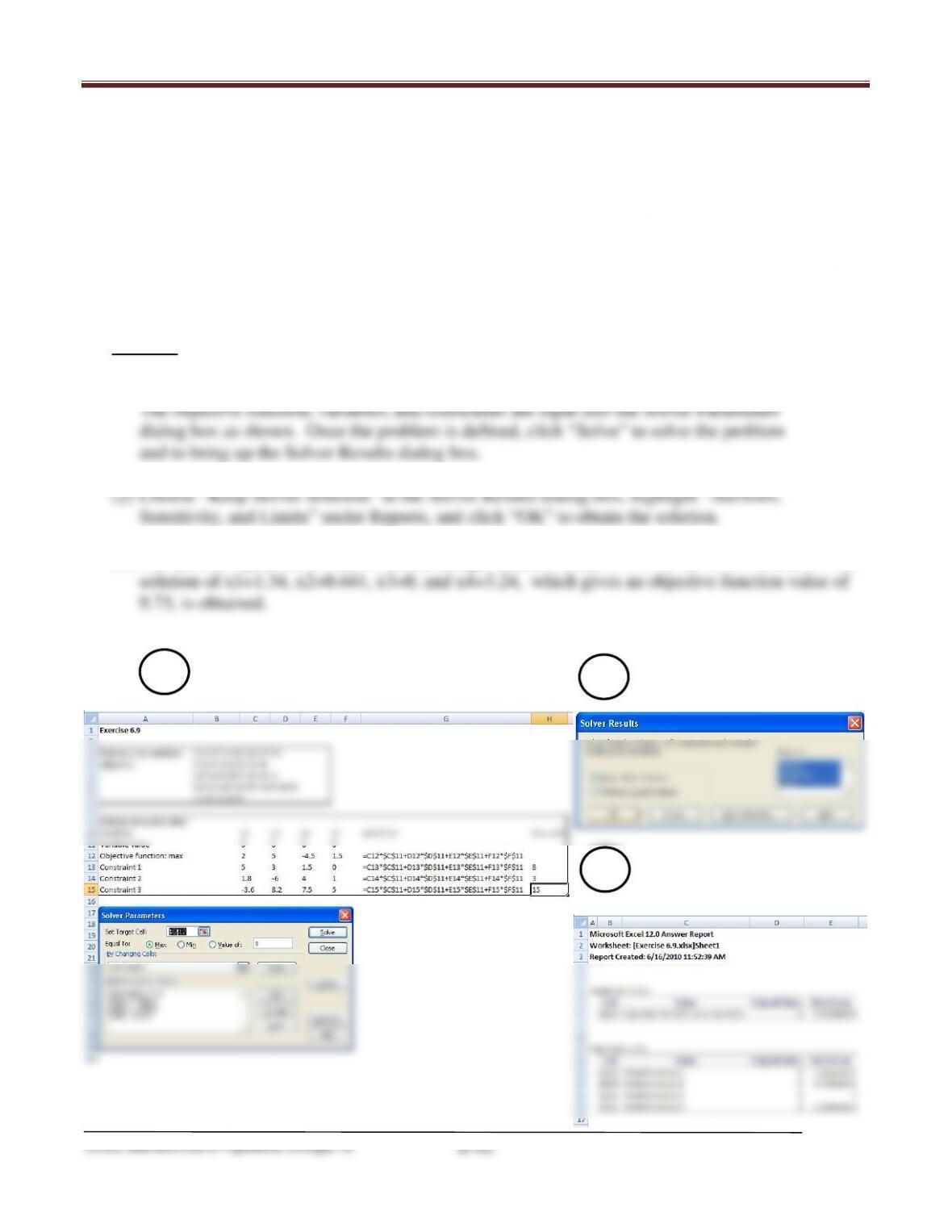
(1) One possible format for setting up the Excel worksheet for this problem is shown below.
(3) The answer report shows that for initial design variable values of x1=0, x2=0, x3=0, and x4=0, a
2
3
1

Chapter 6 Optimum Design: Numerical Solution Process and Excel Solver
Arora, Introduction to Optimum Design, 4e
6-13
Section 6.7 Excel Solver for Nonlinear Programming
Solve the following problems using Excel Solver:
6.12 ________________________________________________________________________________
Solve the following NLP problem using the Excel Solver:
Exercise 3.35 (Exercise 3.34 using inner and outer diameter as design variables)
Design a hollow torsion rod shown in Fig.E3.34 to satisfy the following requirements (created by
J.M. Trummel):
1. The calculated shear stress, , shall not exceed the allowable shear stress under the normal
operation torque To (N·m).
2. The calculated angle of twist, , shall not exceed the allowable twist, (radians).
3. The member shall not buckle under a short duration torque of Tmax (N·m).
Requirements for the rod and material properties are given in Table E3.34(A) and E3.34(B) (select a
material for one rod). Use the following design variables:
x1 = outside diameter of the shaft; x2 = ratio of inside/outside diameter, di/do.
Using graphical optimization, determine the inside and outside diameters for a minimum mass
rod to meet the above design requirements. Compare the hollow rod with an equivalent solid
rod (di/do = 0). Use consistent set of units (e.g. Newtons and millimeters) and let the minimum and
maximum values for design variables be given as
0.02 ≤ ≤0.5 m, 0.60 ≤
≤0.999
Useful expressions for the rod are:
Mass of rod:
=
4(
2−
2),
Calculated shear stress:
=
,
Calculated angle of twist:
=
,
Critical buckling torque:
=
3
12√2(1 − 2)0.75 (1 −
)2.5, N. m
Notation
M = mass of the rod (kg),
= outside diameter of the rod (m),
= inside diameter of the rod (m),
= mass density of material (kg/m3),
l = length of the rod (m),
T0 = Normal operation torque (N
⋅
m),
c = Distance from rod axis to extreme fiber (m),
J = Polar moment of inertia (m4),
θ
= Angle of twist (radians),
G = Modulus of rigidity (Pa),
Chapter 6 Optimum Design: Numerical Solution Process and Excel Solver
Tcr = Critical buckling torque (N
⋅
m),
E = Modulus of elasticity (Pa), and
= Poisson’s ratio.
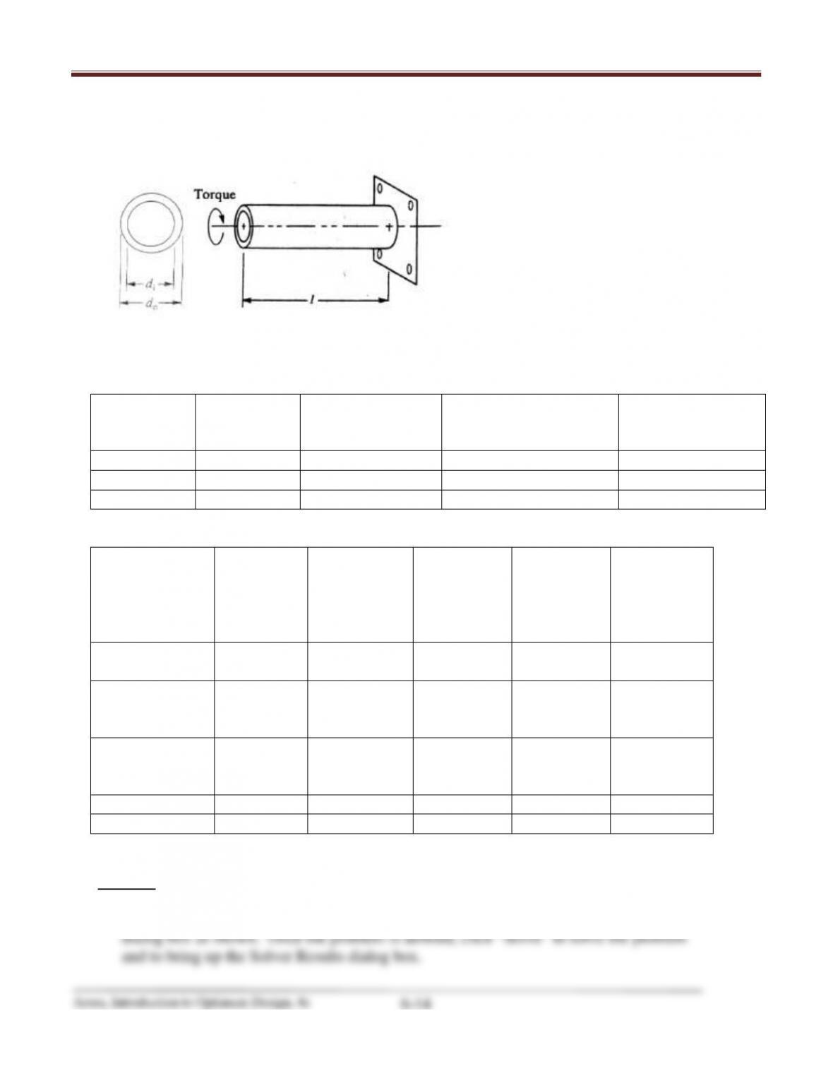
FIGURE E3-34 Hollow torsion rod.
TABLE E3–34(A) Rod Requirements
Torsion
rod
number
Length,
l (m)
Normal torque,
T0 (kN
⋅
m)
Max. torque,
Tmax (kN
⋅
m)
Allowable twist,
(degrees)
1
0.50
10.0
20.0
2
2
0.75
15.0
25.0
2
3
1.00
20.0
30.0
2
TABLE E3–34(B) Materials and Properties for the Torsion Rod
Material
Density,
(kg/m3),
Allowable
Shear
stress,
(MPa)
Elastic
modulus,
E (GPa)
Shear
modulus,
G (GPa)
Poisson’s
ratio (
)
1. 4140
alloy steel
7850
275
210
80
0.30
2.
Aluminum
alloy 24 ST4
2750
165
75
28
0.32
3.
Magnesium
alloy A261
1800
90
45
16
0.35
4. Berylium
1850
110
300
147
0.02
5. Titanium
4500
165
110
42
0.30
Solution
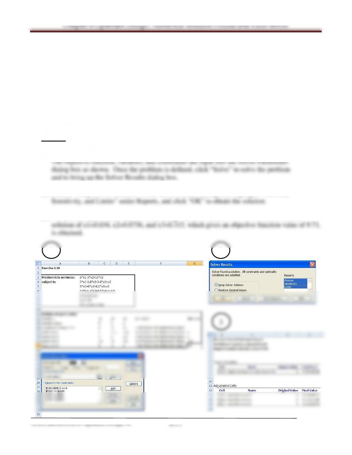
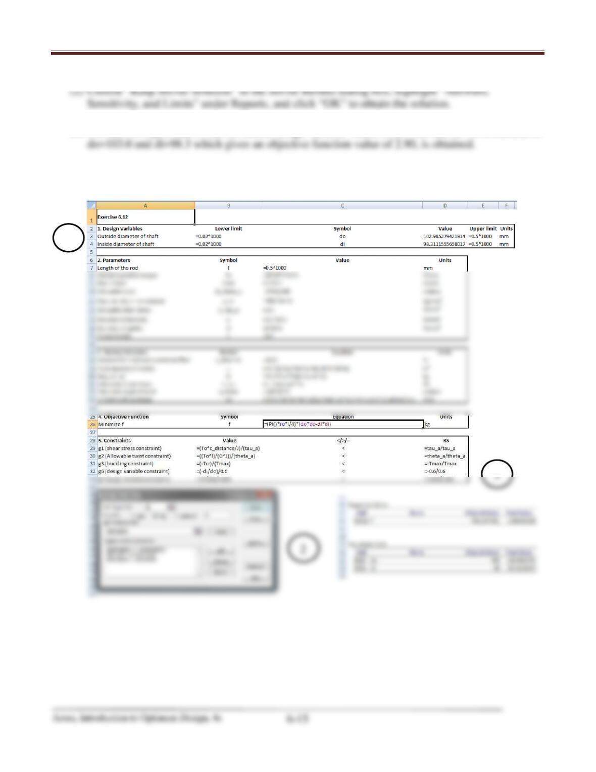
(1) One possible format for setting up the Excel worksheet for this problem is shown below.
The objective function, variables, and constraints are input into the Solver Parameters
Chapter 6 Optimum Design: Numerical Solution Process and Excel Solver
(3) The answer report shows that for initial design variable values of do=400 and di=40 a solution of
1
2
3
Arora, Introduction to Optimum Design, 4e
6-16
6.13 ________________________________________________________________________________
Solve the following NLP problem using the Excel Solver:
Exercise 3.50
A minimum mass structure (area of member 1 is the same as member 3) three–bar truss is to be
designed to support a load P as shown in Fig. 2.9. The following notation may be used: Pu=P cos,
Pv=P sin, A1 = cross–sectional area of members 1 and 3, A2 = cross–sectional area of member 2.
The members must not fail under the stress, and deflection at node 4 must not exceed 2cm in
either direction. Use Newtons and millimeters as units. The data is given as P = 50 kN; = 30°;
mass density, = 7850 kg/m3; modulus of elasticity, E = 210 GPa; allowable stress, = 150 MPa.
The design variables must also satisfy the constraints 50 ≤Ai ≤5000 mm2 .
Solution
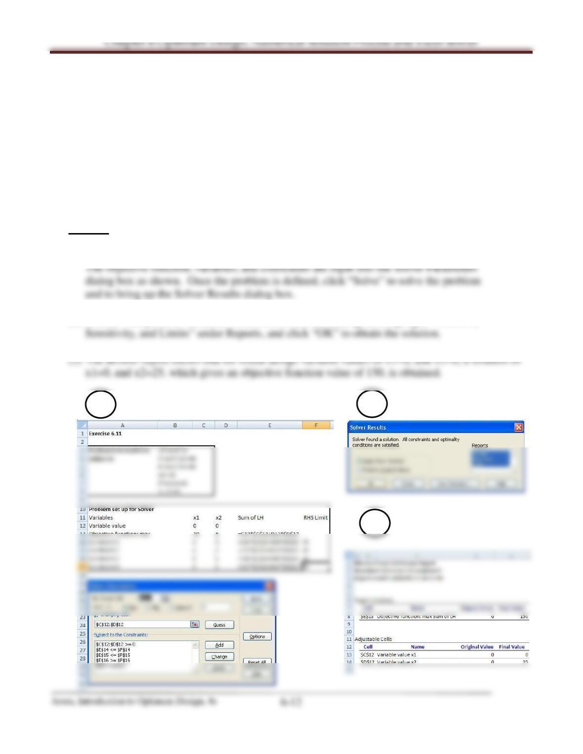
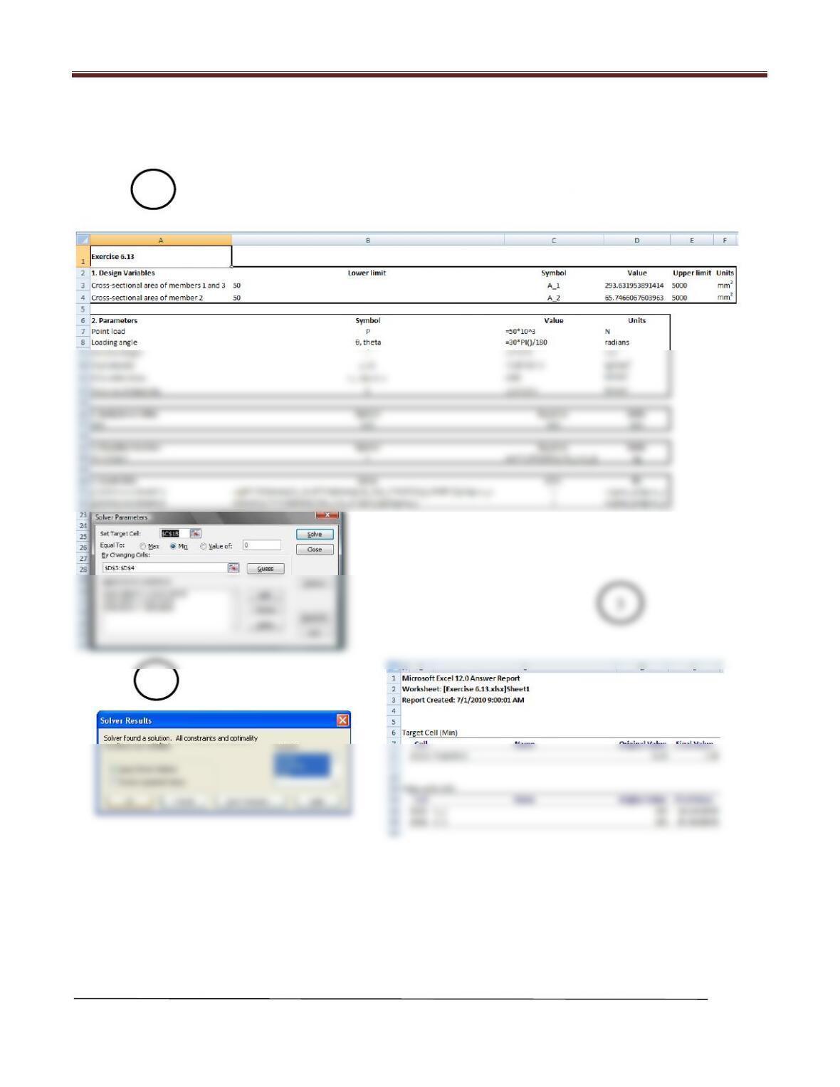
(1) One possible format for setting up the Excel worksheet for this problem is shown below.
Chapter 6 Optimum Design: Numerical Solution Process and Excel Solver
Arora, Introduction to Optimum Design, 4e
6-17
Continued.
3
2
1