Arora, Introduction to Optimum Design, 4e 5-1
CHAPTER
5
More on Optimum Design Concepts:
Optimality Conditions
5.1_________________________________________________________________________________
Answer True or False.
3. The Hessian of the Lagrange function must be positive definite at constrained minimum
4. For a constrained problem, if the sufficiency condition of Theorem 5.2 is violated, the
5. If the Hessian of the Lagrange function at x∗, ∇2L(x∗), is positive definite, the optimum
6. For a constrained problem, the sufficient condition at x∗ is satisfied if there are no
5.2 _________________________________________________________________________________
Formulate the problem of Exercise 4.84. Show that the solution point for the problem is not a regular
point. Write KKT conditions for the problem, and study the implication of the irregularity of the
solution point. Refer to solution of Exercises 4.84:
A refinery has two crude oils:
2. Crude B costs $150/bbl and 30,000 are available.
The company manufactures gasoline and lube oil from the crudes. Yield and sale price barrel of the
product and markets are shown in Table E2.2. How much crude oils should the company use to
maximize its profit? Formulate the optimum design problem.
Table E2.2 Data for Refinery Operation
Chapter 5 More on Optimum Design Concepts: Optimality Conditions
Arora, Introduction to Optimum Design, 4e
5-2
Product
Yield/bbl
Sale Price
per bbl ($)
Market (bbl)
Crude A
Crude B
Gasoline
0.6
0.8
200
20,000
Lube oil
0.4
0.2
450
10,000
Solution
According to the graphical solution, the point P (20000, 10000) is the minimum point with
Referring to the formulation in Exercise 2.2, we have
Minimize
180 100f =– A- B
subject to:
1
g 0 6 0 8 20,000 0AB=+− ≤..
, (gasoline market)
g 0 4 0 2 10,000 0AB=+− ≤..
1 12 2
Chapter 5 More on Optimum Design Concepts: Optimality Conditions
Arora, Introduction to Optimum Design, 4e
5-4
5.4 _________________________________________________________________________________
Solve the following problem graphically. Check necessary and sufficient conditions for candidate
local minimum points and verify them on the graph for the problem.
Minimize (1,2)= 41
2+ 32
2−512−81
subject to 1+2−4 = 0
Solution
Minimize
( )
121
2
2
2
121
8534 , xxxxxxxf −−+=
subject to
12
h 40xx= + −=
;
( )
48534 21121
2
2
2
1−++−−+= xxvxxxxxL
;
The necessary conditions give
1 1 2 2 2 1 12
8 5 8 0; 6 5 0; h 4 0Lx x x v Lx x x v x x∂ ∂= − −+= ∂ ∂ = − += = + −=
The solution of these equations is
.6/1 ,6/11 ,6/13
21
−=== vxx
Therefore, (13/6, 11/6) is a KKT point;
3/52−=f
Check for regularity:
hÑ
= (1, 1). Since
hÑ
is the only vector, regularity of feasible points is
satisfied.
Referring to Exercises 4.43/4.97, the point satisfying the KKT necessary conditions is
Chapter 5 More on Optimum Design Concepts: Optimality Conditions
5.5 _________________________________________________________________________________
Solve the following problem graphically. Check necessary and sufficient conditions for candidate
local minimum points and verify them on the graph for the problem.
Maximize (1,2)= 41
2+ 32
2−512−81
subject to 1+2−4 = 0
Solution
Maximize
( )
121
2
2
2
1
21
8534 , xxxxxxxF −−+=
subject to
12
h 40xx= + −=
;
( )
48534
21121
2
2
2
1
−++++−−= xxvxxxxxL
;
The necessary conditions give
1 1 2 2 2 1 12
8 5 8 0; 6 +5 0; h 4 0Lx x x v Lx x x v x x∂ ∂=− + ++= ∂ ∂ =− += = + −=
The solution of these equations is
.6/1 ,6/11 ,6/13 21 === vxx
Therefore, (2.166667, 1.833333) is a KKT point;
3/52−=F
Check for regularity:
hÑ
= (1, 1). Since
hÑ
is the only vector, regularity of feasible points is
satisfied.
Referring to Exercises 4.44/4.98, the point satisfying the KKT necessary conditions is
Arora, Introduction to Optimum Design, 4e
5-6
5.6 _________________________________________________________________________________
Solve the following problem graphically. Check necessary and sufficient conditions for candidate
local minimum points and verify them on the graph for the problem.
Minimize (1,2)= (1−2)2+ (2+ 1)2
subject to 21+ 32−4 = 0
Solution
Minimize
( ) ( ) ( )
22
12 1 2
, 2 1fxx x x=−++
subject to h=
12
2 3 40xx+ −=
;
( ) ( ) ( )
22
1 2 12
2 1 2 3 4;L x x vx x=− + ++ + −
The KKT necessary conditions give
1 1 2 2 12
2 2 2 0; 2 +1) 3 0; h 2 3 4 0Lx x v Lx x v x x∂∂= −+ = ∂∂= + = = + −=() (
The solution of these equations is
12
32 /13, 4 /13, 6 /13.xx v= =−=−
Therefore, (32/13, -4/13) is a KKT point;
9 /13f=
Check for regularity:
hÑ
= (2, 3). Since
hÑ
is the only vector, regularity of feasible point is
satisfied.
Referring to Exercises 4.45/4.99, the point satisfying the KKT necessary conditions is
x1 = 2.46154, x2 = -0.307692,
v=
-0.46154, f = 0.69231. The point satisfies second order
sufficiency condition.
5.7 _________________________________________________________________________________
Solve the following problem graphically. Check necessary and sufficient conditions for candidate
local minimum points and verify them on the graph for the problem.
Minimize (1,2)= 41
2+ 92
2+ 62−41+13
subject to 1−32+ 3 = 0
Solution
Minimize (1,2)= 41
2+ 92
2+ 62−41+13 subject to h = 1−32+ 3 = 0;
hÑ
hÑ
v=
2+ 92
2+ 62−41+13 +(1−32+ 3)
Chapter 5 More on Optimum Design Concepts: Optimality Conditions
5.8 _________________________________________________________________________________
Solve the following problem graphically. Check necessary and sufficient conditions for candidate
local minimum points and verify them on the graph for the problem.
Minimize ()= (1−1)2+ (2+ 2)2+ (3−2)2
subject to 21+ 32−1 = 0
1+2+ 23−4 = 0
Solution
Minimize
( ) ( ) ( ) ( )
222
12 1 2 3
, 1 2 2fxx x x x=−+ + + −
subject to h1=
12
231xx+−
; h2=
12 3
24xx x++ −
( ) ( ) ( ) ( ) ( )
222
1 2 3 1 1 2 21 2 3
1 2 2 2 3 1 2 4;L x x x v x x vx x x= − + + + − + + −+ + + −
The KKT necessary conditions give
1 1 12 2 2 12 3 3 2
1 1 2 2 12 3
2 1 2 0; 2 +2) 3 0; 2 –2) 2 0
h 2 3 1 0h 2 4 0
Lx x v v Lx x v v Lx x v
x x xx x
∂∂= −+ += ∂∂= + += ∂∂= + =
= + −= = + + − =
() ( ( ;
;
The solution of these equations is
12 3
1.71698, 0.81132, 1.547170057xx x= =−=
12
0.943396132, 0.452829943vv=−=
Therefore, (1.71698066, -0.811320724, 1.547170057) is a KKT point;
2.1318f=
Check for regularity: Gradients of the constraints are linearly independent; therefore the point is
a regular point of the feasible set.
Referring to Exercises 4.47/4.101, the point satisfying the KKT necessary conditions is
x1 = 1.71698, x2 = -0.81132, x3 = 1.54714,
v=
1
-0.943396,
v=
2
0.4528299, f = 2.11318. The point
satisfies second order sufficiency condition.
5.9 _________________________________________________________________________________
Solve the following problem graphically. Check necessary and sufficient conditions for candidate
local minimum points and verify them on the graph for the problem.
Minimize (1,2)= 91
2+1812+132
2−4
subject to 1
2+2
2+ 21−16 = 0
Solution
Minimize
( )
413189 , 2
221
2
121 −++= xxxxxxf
subject to
22
12 1
h 2 16 0xx x=++ −=
( )
( )
2 2 22
1 2 1 12 2 1 2 1
1121 2 1 21
22
12 1
, , 9 18 13 4 2 16
18 18 2 2 0; 18 26 2 0
h 2 16 0
L x x v x xx x v x x x
L x x x vx v L x x x vx
xx x
= + + −+ + + −
∂∂= + + + = ∂∂ = + + =
=++ −=
;
These equations are nonlinear, which can be solved numerically. Using any nonlinear equation
solver, we can find the following KKT points:
12
Check for regularity:
( )
12
h 2 2, 2xx= +Ñ
. Since
hÑ
is the only vector, regularity of feasible
points is satisfied for each KKT point.
Arora, Introduction to Optimum Design, 4e
5-9
5.10 ________________________________________________________________________________
Solve the following problem graphically. Check necessary and sufficient conditions for candidate
local minimum points and verify them on the graph for the problem.
Minimize (1,2)= (1−1)2+ (2−1)2
subject to 1+2−4 = 0
Solution
Minimize
( ) ( )
2
2
2
111 −+−= xxf
subject to
12
h 40xx= + −=
(
) ( ) ( )
411 21
2
2
2
1−++−+−= xxvxxL
; the KKT necessary conditions are
( ) ( )
1 1 2 2 12
2 1 0; 2 1 0; h 4 0Lx x v Lx x v x x∂∂ = − += ∂∂ = − += = + −=
Solution of these equations is
2
,2 ,2 21 −=== vxx
. Therefore,
( )
2 ,2
is a KKT point; f = 2.
Check for regularity:
( )
h 1, 1=Ñ
. Since
hÑ
is the only vector, regularity of feasible points is
satisfied.
Refer to Exercises 4.49/4.103
( )
2 ,2
is a KKT point; f = 2. The point satisfies second order necessary conditions.
Chapter 5 More on Optimum Design Concepts: Optimality Conditions
5.11 _______________________________________________________________________________
Solve the following problem graphically. Check necessary and sufficient conditions for candidate
local minimum points and verify them on the graph for the problem.
Minimize (1,2)= 41
2+ 32
2−512−8
subject to 1+2= 4
Solution
Minimize
22
1 2 12
435 8fxxxx=+− −
subject to
12
h 40xx= + −=
( )
22
1 2 12 1 2
435 8 4Lxxxx vxx= + − −+ + −
; the KKT necessary conditions are
1 1 2 2 2 1 12
8 5 0; 6 5 0; h 4 0Lx x x v Lx x x v x x∂∂ = − += ∂∂ = − += = + −=
Solution of these equations is
12
11/ 6, 13 / 6, 23 / 6xx v= = = −
.
Therefore,
( )
11/ 6, 13 / 6
is a KKT point; f* = -1/3.
Check for regularity:
( )
h 1, 1=Ñ
. Since
hÑ
is the only vector, regularity of feasible point is
satisfied.
Referring to Exercises 4.51/4.105, the point satisfying the KKT necessary conditions is
x1 = 1.83333, x2 = 2.16667,
v=
-3.83333, f = -0.33333. The point satisfies second order sufficiency
condition. The sufficiency check is same as in Exercise 5.5.
Arora, Introduction to Optimum Design, 4e
5-11
5.12 _______________________________________________________________________________
Solve the following problem graphically. Check necessary and sufficient conditions for candidate
local minimum points and verify them on the graph for the problem.
Maximize (1,2)= 41
2+ 32
2−512−8
subject to 1+2= 4
Solution
Minimize
22
1 2 12
435 8f x x xx=−− + +
subject to
12
h 40xx= + −=
( )
22
1 2 12 1 2
435 8 4L x x xx v x x=− − + ++ + −
The KKT necessary conditions are
1 1 2 2 2 1 12
8 5 0; 6 5 0; h 4 0Lx x x v Lx x x v x x∂∂ =− + += ∂∂ =− + += = + −=
Solution of these equations is
12
11/ 6, 13 / 6, 23 / 6xx v= = =
.
Chapter 5 More on Optimum Design Concepts: Optimality Conditions
5.13 _______________________________________________________________________________
Solve the following problem graphically. Check necessary and sufficient conditions for candidate
local minimum points and verify them on the graph for the problem.
Maximize (1,2)= 41
2+ 32
2−512−8
subject to 1+2≤4
Solution
Minimize
22
1 2 12
435 8f x x xx=−− + +
subject to
12
g 40xx= + −≤
( )
22 2
1 2 12 1 2
435 8 4L x x xx u x x s=− − + ++ + −+
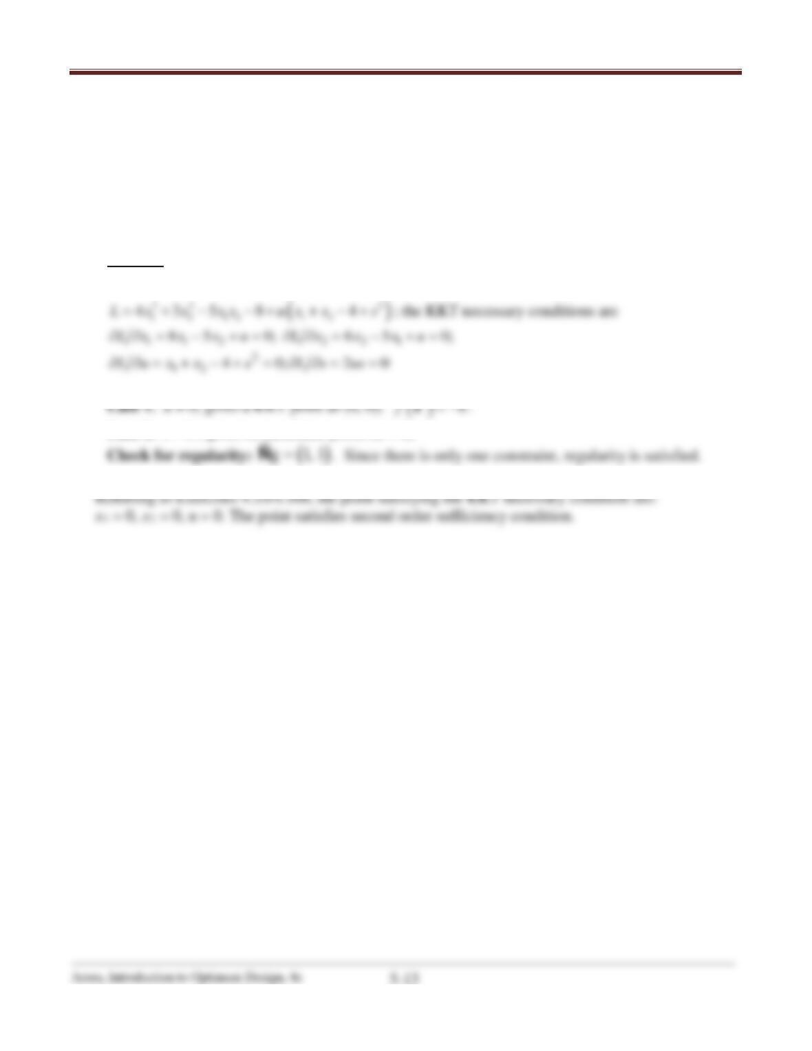
; the KKT necessary conditions are
1 12 2 21
2
12
8 5 0; 6 5 0;
4 0; 2 0
Lx x x u Lx x x u
Lu x x s Ls us
∂∂=− + += ∂∂ =− + +=
∂∂= + −+ = ∂∂= =
Chapter 5 More on Optimum Design Concepts: Optimality Conditions
5.14 _______________________________________________________________________________
Solve the following problem graphically. Check necessary and sufficient conditions for candidate
local minimum points and verify them on the graph for the problem.
Minimize (1,2)= 41
2+ 32
2−512−8
subject to 1+2≤4
Solution
Minimize
22
1 2 12
435 8fxxxx=+− −
subject to
12
g 40xx= + −≤
( )
22 2
1 2 12 1 2
435 8 4Lxxxx uxx s= + − −+ + −+
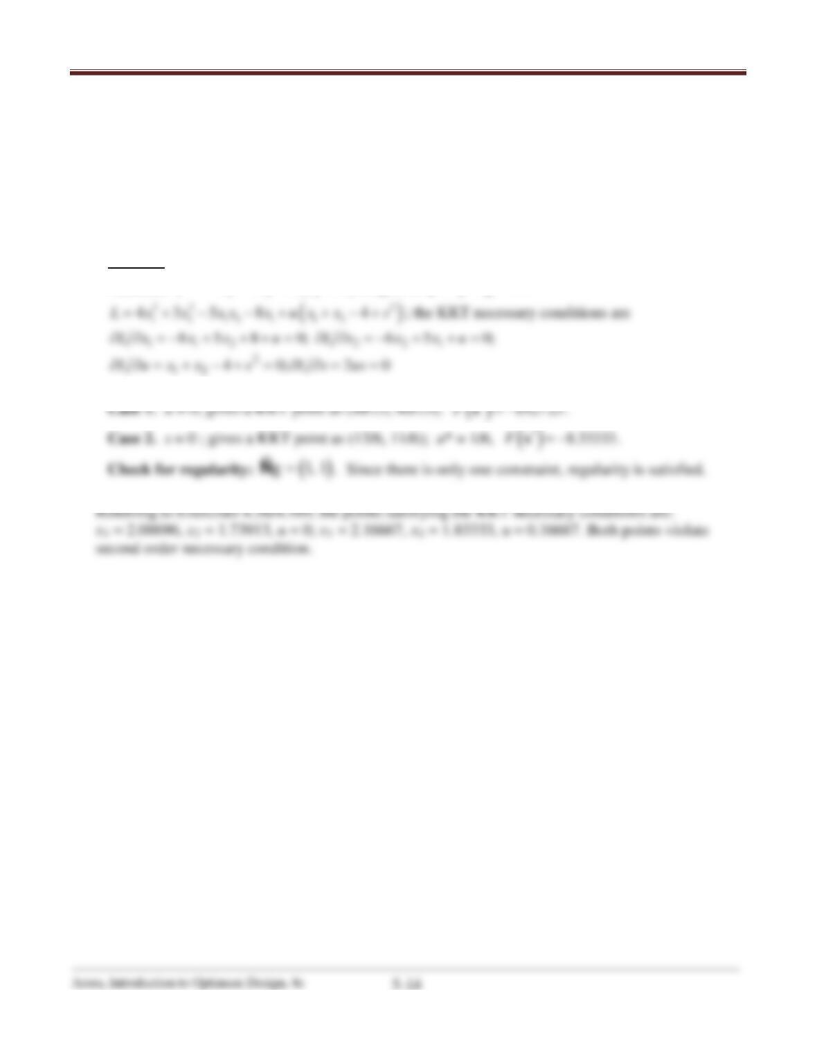
; the KKT necessary conditions are
112 2 21
2
12
8 5 0; 6 5 0;
4 0; 2 0
Lx x x u Lx x x u
Lu x x s Ls us
∂∂= − += ∂∂ = − +=
∂∂= + −+ = ∂∂= =
∗
Chapter 5 More on Optimum Design Concepts: Optimality Conditions
5.15 _______________________________________________________________________________
Solve the following problem graphically. Check necessary and sufficient conditions for candidate
local minimum points and verify them on the graph for the problem.
Maximize (1,2)= 41
2+ 32
2−512−81
subject to 1+2≤4
Solution
Minimize
22
1 2 12 1
435 8f x x xx x=−− + +
subject to
12
g 40xx= + −≤
( )
22 2
1 2 12 1 1 2
435 8 4Lxxxxxuxx s= + − − + + −+
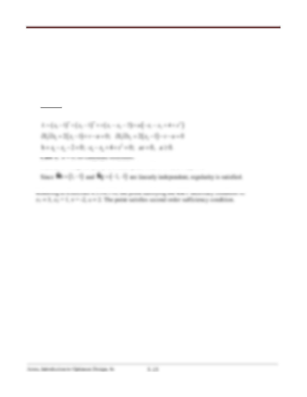
; the KKT necessary conditions are
1 12 2 21
2
12
8 5 8 0; 6 5 0;
4 0; 2 0
Lx x x u Lx x x u
Lu x x s Ls us
∂∂=− + ++= ∂∂ =− + +=
∂∂= + −+ = ∂∂= =
∗
Chapter 5 More on Optimum Design Concepts: Optimality Conditions
5.16 _______________________________________________________________________________
Solve the following problem graphically. Check necessary and sufficient conditions for candidate
local minimum points and verify them on the graph for the problem.
Minimize (1,2)= (1−1)2+ (2−1)2
subject to 1+2≥4
1− 2−2 = 0
Solution
Minimize
( ) ( ) ( )
22
12
11fx x x=−+ −
; subject to
12
h 2 0;xx= − −=
12
g 40xx=−− +≤.
( ) ( ) ( )
( )
22 2
1 2 12 12
11 2 4L x x vxx uxx s= − + − + −−+−−++
( ) ( )
11 2 2
2 1 0; 2 1 0Lx x vu Lx x vu∂∂= − +−= ∂∂ = − −−=
2
12 12
h 2 0; – 4 0; 0, 0.xx xx s us u=−−= −++= = ≥
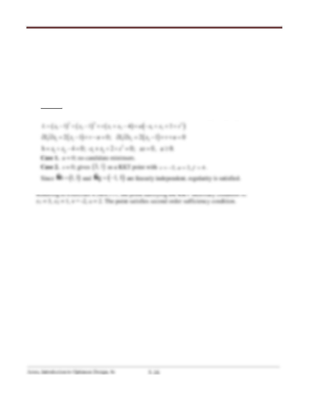
Case 1. u = 0; no candidate minimum.
Case 2. s = 0; gives
( )
3, 1
as a KKT point with
2, 2, 4v uf=−= =
.
Chapter 5 More on Optimum Design Concepts: Optimality Conditions
5.17 _______________________________________________________________________________
Solve the following problem graphically. Check necessary and sufficient conditions for candidate
local minimum points and verify them on the graph for the problem.
Minimize (1,2)= (1−1)2+ (2−1)2
subject to 1+2= 4
1− 2−2≥0
Solution
Minimize
( ) ( ) ( )
22
12
11fx x x=−+ −
; subject to
12
h 4 0;xx= + −=
12
g 20xx=−+ +≤.
( ) ( ) ( )
( )
22 2
1 2 12 12
11 4 2L x x vxx uxx s= − + − + +−+−+++
( ) ( )
11 2 2
2 1 0; 2 1 0Lx x vu Lx x vu∂ ∂ = − +− = ∂ ∂ = − ++ =
2
12 12
h 4 0; – 2 0; 0, 0.xx xx s us u=+−= +++= = ≥
Case 1. u = 0; no candidate minimum.
Case 2. s = 0; gives
( )
3, 1
as a KKT point with
2, 2, 4v uf=−= =
.
Since
( )
h 1, 1=Ñ
and
( )
g 1, 1= −Ñ
are linearly independent, regularity is satisfied.
Chapter 5 More on Optimum Design Concepts: Optimality Conditions
Arora, Introduction to Optimum Design, 4e
5-17
5.18 _______________________________________________________________________________
Solve the following problem graphically. Check necessary and sufficient conditions for candidate
local minimum points and verify them on the graph for the problem.
Minimize (1,2)= (1−1)2+ (2−1)2
subject to 1+2≥4
1− 2≥2
Solution
Minimize
( ) ( ) ( )
22
12
11fx x x=−+ −
; subject to
1 12
g 4 0;xx=−− +≤
2 12
g 20xx=−+ +≤.
( ) ( )
( ) ( )
22 22
1 2 1 12 1 2 12 2
11 4 2Lx x uxxsuxxs= − + − + − − ++ + − + ++
( ) ( )
1 1 12 2 2 12
2 1 0; 2 1 0Lx x u u Lx x u u∂∂= −− − = ∂∂= −− + =
22
1 2 1 1 2 2 11 2 2 1 2
4 0; – 2 0; 0, 0, 0.xxs xxs usus uu− − ++ = + ++ = = = ≥,
Case 1. u1 = 0, u2 = 0; no candidate minimum.
Case 2. u1 = 0, s2 = 0; no candidate minimum.
Case 4. s1 = 0, s2 = 0; gives
( )
3, 1
as a KKT point with
12
2, 2, 4uuf= = =
.
Chapter 5 More on Optimum Design Concepts: Optimality Conditions
5.19 _______________________________________________________________________________
Solve the following problem graphically. Check necessary and sufficient conditions for candidate
local minimum points and verify them on the graph for the problem.
Minimize (,)= ( − 4)2+ ( − 6)2
subject to 12 ≥ +
≥ 6, ≥ 0
Solution
Minimize
( ) ( )
22
(, ) 4 6f xy x y=− +−
;
3
( ) ( )
( ) ( ) ( )
22 2 22
1 1 2 23 3
4 6 12 6Lx y uxy sux suys=−+−+ +−++−+++−+
( )
( )
12
13
2 4 0;
26 0
Lx x u u
Ly y u u
∂ ∂= − + − =
∂ ∂= − + − =
2
1
2
2
2
3
11 2 2 3 3
123
12 0;
6 0;
y 0
0, 0, 0
0.
xy s
xs
s
us us us
uuu
+− + =
−+ + =
−+ =
= = =
≥,,
Case 2.
12 3
0, 0uu s= = =
; no candidate minimum.
Case 3.
13 2
0, 0uu s= = =
; gives
( )
6, 6
as a KKT point with
2 13
4, s =0, s =6, 4uf= =
.
Case 5.
1 23
0, 0u ss= = =
; no candidate minimum.
Case 7.
3 12
0, 0u ss= = =
; gives
( )
6, 6
as a KKT point with
123
0, 4, s 6, 4uu f= = = =
.
Chapter 5 More on Optimum Design Concepts: Optimality Conditions
5.20 ________________________________________________________________________________
Solve the following problem graphically. Check necessary and sufficient conditions for candidate
local minimum points and verify them on the graph for the problem.
Minimize (1,2)= 21+ 32− 1
3−22
2
subject to 1+ 32≤6
51+ 22≤10
1,2≥0
Solution
( )
32
1 21 2
Minimize 2 3 2 ;
f x xx x
= + −−
x
g2 =
424.−
< 0, g3 =
8160.−
< 0, g4 =
750.−
< 0. All the KKT conditions are satisfied; therefore
Case 8.
;0 ,0 3241 ==== ssuu
gives no candidate point.
Case 9.
;0 ,0 4132 ==== ssuu
gives no candidate point.
Case 10.
2 4 13
0, 0;uu ss= = = =
gives
( )
2 ,0
as a KKT point with
311 ,35
31
== uu
,
2−=f
.
;0 ,0 2143 ==== ssuu
0 ,0
Case 15.
0 ,0
3214
==== sssu
; gives no candidate point.