Chapter 5 More on Optimum Design Concepts: Optimality Conditions
5.67 ________________________________________________________________________________
The formulation is given in Exercise 3.35*. Optimum solution and check of necessary and sufficient
conditions can be found in Exercise 5.46.
Rewriting the formulation of Exercise 3.35, we have
223
−
7 44
Chapter 5 More on Optimum Design Concepts: Optimality Conditions
Arora, Introduction to Optimum Design, 4e
5-76
5.68 ________________________________________________________________________________
The formulation is given in Exercise 3.36*. Optimum solution and check of necessary and sufficient
conditions can be found in Exercise 5.47.
Rewriting the formulation of Exercise 3.36, we have
Minimize
0.02466f Rt=
, subject to
( )
( )
( )
6 33
1
3.1831 10 2 4 275 0;g R t R t Rt= × + + −≤
( ) ( ) ( )
( )
05
4 3 3 2 7 5 25
23
3 97886 10 4 3 49066 10 0; 2 0 10 3 37972 10 0 5 0;
..
. . .. .g R t Rt g R t t
−
= × + − × ≤ =×− × + ≤
4
50 0;gR= −≤
5 67
200 0; 2 0; 40 0gR g t gt= − ≤ = −≤ =− ≤
The optimum solution obtained by the graphical method is
92 ,342 ,350 .f.t.R === ∗∗∗
where g1
and g3 are active.
24567
0.uuuuu= = = = =
( )
( )
( )
6 33
1
0 02466 3 1831 10 2 4..
t
L R u R t R t Rt
= + ×+ +
( )
( )
05
7 5 25
3
2 0 10 3 37972 10 0 5
..
.. .u R tt
+ ×− × +
The KKT necessary conditions are
( ) ( )
( )
( ) ( )
2
6 33 23 33
1
0 02466 3 1831 10 2 4 2 12 4..L R t u R t Rt R t R t R t Rt
∂∂= + × + − + + +
( )
( )
( )
05
5 25
1
32
3 37972 10 0 5 0
.
.
..u tR t
− × +=
(1)
( ) ( )
( )
( ) ( )
2
6 33 3 2 33
1
0 02466 3 1831 10 1 4 2 4 3 4..L t R u R t Rt R t R Rt R t Rt
∂ ∂= + × + − + + +
( )
( )
( )
( )
( )
05
5 25 15
1
34
3 37972 10 0 5 2 5 0 5 0u tRt tRt
− × ++ + =
.
..
. .. .
(2)
0, 0, 0
i ii i
g ug u≤=≥
; i = 1 to 7 (3)
Substituting the optimum value into (1) and (2) respectively, we obtain u1 =
3
106434
−
×.
> 0, u3 =
8
102403
−
×.
> 0 (o.k.). All the other conditions in (3) are also satisfied. Therefore, the point obtained
2. Check for sufficient condition. Since the number of active constraints is equal to the number of
design variables, the point
( )
342 ,350 .t.R ==
∗∗
is indeed an isolated local minimum point. The
sufficient condition is deemed satisfied at this point.
The Lagrange multipliers of active constraints are
3
8
11 3 3 1 3
Chapter 5 More on Optimum Design Concepts: Optimality Conditions
5.69 ________________________________________________________________________________
(a) Referring to the formulation in Exercise 3.39 (3.23), we have
43
25 10 0 26045 0;.g Rt=×− ≤
34
50 0; 10 0;g Rt g R= − ≤ = −≤
5 67
1000 0; 5 0; 200 0gR g t gt= − ≤ = −≤ =− ≤
The optimum solution is obtained by the graphical method is R
∗
= 33.7, t
∗
= 5.0,
f
∗
= 41.6 where
g2 and g6 are active.
1. Check for necessary conditions.
Since only g2 and g6 are active, we can set u1 = u3 = u4 = u5 = u7 = 0.
( )
43
26
0 2466 5 10 0 26045 5..L Rt u R t u t
= + ×− + −
∗
∗
2. Check for sufficient condition. Use the same argument as in Exercise 5.53.
3. The effect of variations in constraint limits on cost function
4
22 66 2 6
Δ 2.779 10 5.54f ue ue e e
−
=−−=− × −
(b) Referring to the formulation in Exercise 3.42 (3.24), we have
22
22
1. Check for necessary conditions.
Since only g2 and g4 are active, we can set u1 = u3 = u5 = u6 = u7 = 0.
22 5 44
io R.R
conditions.
2. Check for sufficient condition. Use the same argument as in Exercise 5.53.
3. The effect of variations in constraint limits on cost function
4
22 44 2 4
Δ 2.807 10 5.467f ue ue e e
−
=−−=− × −
5.70 ________________________________________________________________________________
(a) Referring to the formulation in Exercise 3.40 (3.23), we have
1
43
2
34
50 0; 10 0;g Rt g R=− − ≤ = −≤
5 67
1000 0; 5 0; 200 0gR g t gt= − ≤ = −≤ =− ≤
The optimum solution obtained by the graphical method is R
∗
= 21.3, t
∗
= 5.0, f
∗
= 26.0 where g2
and g6 are active.
1. Check for necessary condition.
Since only g2 and g6 are active, we can set u1 = u3 = u4 = u5 = u7 = 0.
L = 0.2466Rt + u2 (5
tR. 34 04181110 −×
) + u6 (5
t−
)
The KKT necessary conditions are:
( )
tR.ut.RL
2
2
12543324660 −=∂∂
= 0;
( )
6
3
2
04181124660 uR.uR.tL −−=∂∂
= 0;
0,0
i
=≤
ii
g ug
,
;0
i≥u
i = 1 to 7
Substituting the optimum values, we obtain u2 = 1.739
4
10
−
×
> 0, u6 = 3.491 > 0 (o.k.). All the other
conditions are also satisfied. Thus, the point (R * = 21.3, t * = 5.0) satisfies the necessary conditions.
2. Check for sufficient condition. Use the same argument as in Exercise 5.53.
3. The effect of variations in constraint limits on cost function
4
22 66 2 6
Δ 1.739 10 3.491f ue ue e e
−
=−−=− × −
(b) Referring to the formulation in Exercise 3.43(3.24), we have
≤
22
io
22
io
g2 = 5
( )
( ) ( )
4 44
3
10 0.26045 0; 2 50 0;
o i oi oi
RR g RR RR× − − ≤ = + − −≤
g4 =
( )
56
5 0; 200 0; 0.5 10 0;
io oi oi
RR g R R g R R− +≤ = − − ≤ =− + + ≤
g7 = 0.5
( )
−+
io
RR
1000
≤
0;
The optimum solution obtained by the graphical method is
024.R
o
=
∗
,
019.R
i
=
∗
, f * = 26.0 where g2
and g4 are active.
1. Check for necessary conditions.
Since only g2 and g4 are active, we can set u1 = u3 = u5 = u6 = u7 = 0.
L = 0.1233(
22
io
RR −
) + u2[5
( )
44
o
4
R26045010
i
R. −−×
] + u4(Ri – Ro+5)
024.R
=
∗
=
∗
2. Check for sufficient conditions. Use the same argument as in Exercise 5.53.
3. The effect of variations in constraint limits on cost function
4
22 44 2 4
Δ 1 699 10 3 471f ue ue e e
−
=−− =− × −..
5.71 ________________________________________________________________________________
(a) Referring to the formulation in Exercise 3.41 (3.23), we have
Minimize f = 0.2466Rt, subject to g1
=
7957.7/(Rt) – 250
≤
0;
43
1. Check for necessary conditions.
Since only g2 and g6 are active, we can set u1 = u3 = u4 = u 5 = u 7 = 0.
L = 0.2466Rt + u2 (5
−× 4
10
0.52091R3t) + u6 (5 – t)
2. Check for sufficient condition. Use the same argument as in Exercise 5.53.
3. The effect of variations in constraint limits on cost function
4
22 66 2 6
Δ 2.065 10 4.439 .f ue ue e e
−
=−− =− × −
(b) Referring to the formulation in Exercise 3.43 (3.24), we have
22
22
5.72 _______________________________________________________________________________
Referring to the formulation in Exercise 3.46, we have
×
3
subject to g1 = (202.97A1+512.95A2)/( A1A2) – 50
≤
0; g2 = 103420/A1 – 250
≤
0;
g3 = A1 – 5000
≤
0; g4 = 40925/ A2 – 250
≤
0; g5 = A2 – 5000
≤
0;
The optimum solution obtained by the graphical method is A
∗
1
= 413.68, A
∗
2
= 163.7, f * = 5.7 where
g2 and g4 are active.
1. Check for necessary conditions. Since only g2 and g4 are active, we can set u1 = u3 = u5 = 0.
L = 9.8125
( )
( )
( )
3
12 2 1 4 2
10 103420 250 40925 250AA u A u A
−
× ++ − + −
The KKT necessary conditions are:
( )
;01034201081259
2
12
3
1
=−×=∂∂
−
Au.AL
( )
;01034201081259
2
12
3
1
=−×=∂∂
−
Au.AL
0 ,0 ,0
ii
≥≤≤ ugug
ii
; i =1 to 5
From the equations, we get u2 = 1.6237
,10
2−
×
u4 = 6.425
3
10−
×
> 0 (o.k.). All the conditions are
∗
∗
Chapter 5 More on Optimum Design Concepts: Optimality Conditions
5.73 _______________________________________________________________________________
≤
53
23
1.034188 10 4.16726 0; 50 0;g Rt g Rt= × − ≤ = −≤
4 5 67
20 0; 400 0; 2 0; 40 0g R gR g t gt= − ≤ = − ≤ = −≤ =− ≤
The optimum solutions obtained by the graphical method are the points on the line segment between
“a” and “b”. We shall check the point “a” where R* = 20. , t* = 3.3 together with g1 and g4 active.
1. Check for necessary conditions.
The KKT necessary conditions are:
2
14
0.1233 16459.5 0;L R t u Rt u
∂∂= − − =
2
1
0.123 16459.5 0; L t R u Rt
∂ ∂= − =
0, 0; 0
i ii i
g ug u≤=≥
; i = 1 to 7
Substituting the optimum values, we get u1 = 0.03263 > 0, u4 = 0
≥
0 (o.k.). All the other conditions
are also satisfied. Thus, the point (R* = 20, t* = 3.3) satisfies the necessary conditions.
2. Check for sufficient condition. We shall consider the general case where only g1 is active. The
Hessian of Lagrangian is
( )( ) ( )
( ) ( )( )
11
3 22
2
11
22 3
16459.5 2 16459.5
0.1233
16459.5 16459.5 2
0.1233
uu
Rt Rt
Luu
R t Rt
+
=
+
Ñ
( )
2
11
2
16459 5 ; 0 gives 1, , 0
16359 5
T
T
Rt
g g c tR c
Rt
= = =−≠
−
.dd .
.
ÑÑ
Hence Q =
2T
LdÑ
d = 0. Thus,
the sufficient condition is not satisfied.
3. The effect of variations in constraint limits on cost function.
11 1
Δ 0 03263.f ue e=−=
10−
×
5.74 _______________________________________________________________________________
Referring to the formulation in Exercise 3.48, we have
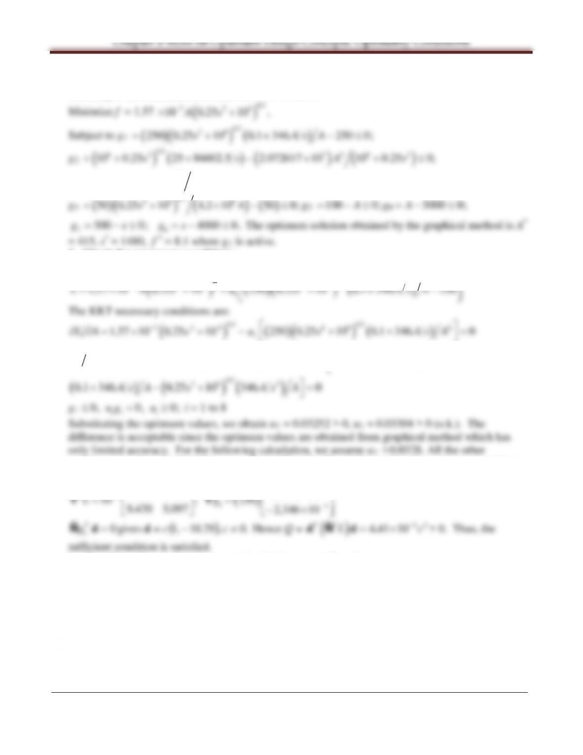
Minimize f = 1.57
5
10−
×
A(h2+5.625
5
10×
)1/2,
1
25
2
Check for necessary conditions. Since only g1 and g7 are active, we can set
u2 = u3 = u4 = u6 = u8 = 0.
L = 1.57
( )
1
52 5
2
10 5 625 10.Ah
−
× +×
( )
( )
( )
1
25
2
1250 5 625 10 100 0 2309 250..uh h A
+ +× + −
1
( )
( )
1
52 5
2
1
1 57 10 5 625 10 250..L h Ah h u
−
−
∂ ∂= × + × +
11
25 252
22
7
−
gi
≤
0, uigi = 0, ui
≥
0; i = 1 to 8
2
−
3
Arora, Introduction to Optimum Design, 4e
5-83
5.75________________________________________________________________________________
Referring to the formulation in Exercise 3.49, we have
05
5 26
.
−
g3
( )
( ) ( )
( )
15
26 2
50 0 25 10 60 62 50 0;
.
..s As= + −≤
15
26 8
.
1. Check for necessary conditions.
The only active constraint is g1, so we can set u2 = u3 = u4 = u5 = u6 = u7 = u8 = 0.
( )
( )
( )
( )
105
5 26 26
2
1
1 57 10 0 25 10 250 0 25 10 0 1 346 4 250
.
. . . ..L A s u s sA
−
=× ++ + + −
The KKT necessary conditions are:
05
5 26
1
.
−
05
26 2
.
( )
( )
( )
05
5 26
1
1 57 10 0 25 0 25 10 250
.
. ..Ls A s s u
−
−
∂ ∂= × + +
( )
05
26
0 25 0 25 10
.
..ss
−
+
( )
( ) ( )
05
26 2
0 1 346 4 0 25 10 346 4 0
.
.. . .sA s s A
+ −+ =
gi
0, 0, 0;
ii i
ug u≤=≥
i = 1 to 8
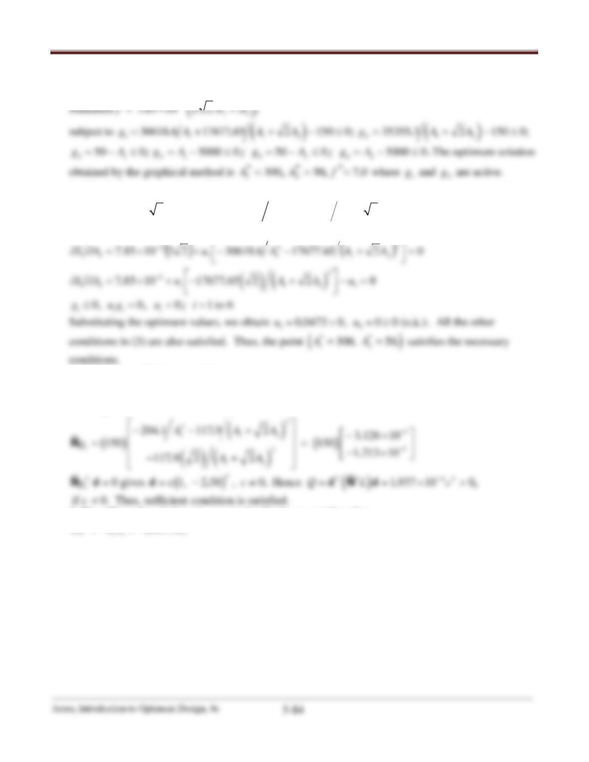
Substituting the optimum values, we obtain u1 = 0.03252 > 0, u1 = 0.03304 > 0 (o.k.). The
difference is acceptable since the optimum values are obtained from graphical method which has
only limited accuracy. For the following calculation, we assume u1
=
0.0328. All the other
conditions are also satisfied. Thus, the point (A* = 415, s* = 1480) satisfies the necessary conditions.
2. Check for sufficient condition.
( )
3
26
14
9 535 9 420 2 413 10
10 ; 250
9 420 5 097 2 346 10
.. .
.. .
Lg
−
−
−
−×
= =
−×
∇∇
1
0
T
g=dÑ
gives d = c
( )
.c. 0 ,2910 ,1 ≠−
Hence Q =
( )
2 42
4 41 10
T
Lc
−
= ×d d.Ñ
> 0. Thus, the
sufficient condition is satisfied.
3. The effect of variations in constraint limits on cost function
11 1
Δ 0 0328.f ue e=−=−
Chapter 5 More on Optimum Design Concepts: Optimality Conditions
5.76________________________________________________________________________________
Referring to the formulation in Exercise 3.50, we have
3
−
5.77________________________________________________________________________________
Referring to the formulation in Exercise 3.51, we have
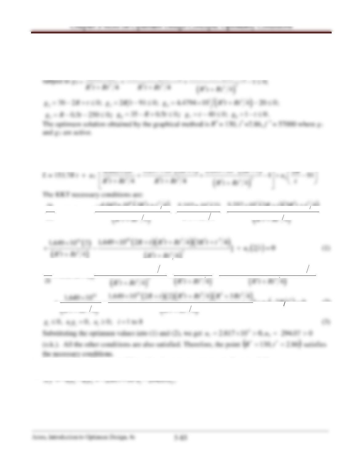
Minimize f = 153.7R t,
( ) ( )
3 10
6
5 257 10 2 1 649 10 2
4 045 10 1 0;
Rt Rt
×+ × +
×
..
.
1. Check for necessary conditions.
Since only g1 and g3 are active, we can set u2 = u4 = u5 = u6 = u7 = u8 = 0.
( ) ( )
3 10
6
5 257 10 2 1 649 10 2
4 045 10 2
..
.Rt Rt R
×+ × +
×
5.78________________________________________________________________________________
Referring to the formulation in Exercise 3.52, we have
Minimize f = 6.126
( )
22
,
oi
dd−
subject to
( )
8
4
144
1 42603 10 1 65 10 0;
..
o
oi
d
gdd
×
= − ×≤
−
( )
( ) ( )
22 6
23
44 44
40743 7 3 719 10
5000 0; 10 0
..;
o oi i
oi oi
d dd d
gg
dd dd
++ ×
= − ≤ = −≤
−−
( )
( ) ( ) ( )
4 56
600 20 05 20
2
; ;. ;
oi oi
oi
oi
dd dd
g g g dd
dd
+−
= − ≤ = −≤ = − + ≤
−
7 8 9 10
50 0 5 0 45 0 4 0;; ;.
o oi i
gd g d gd g d= − ≤ =− ≤ =− ≤ =−≤
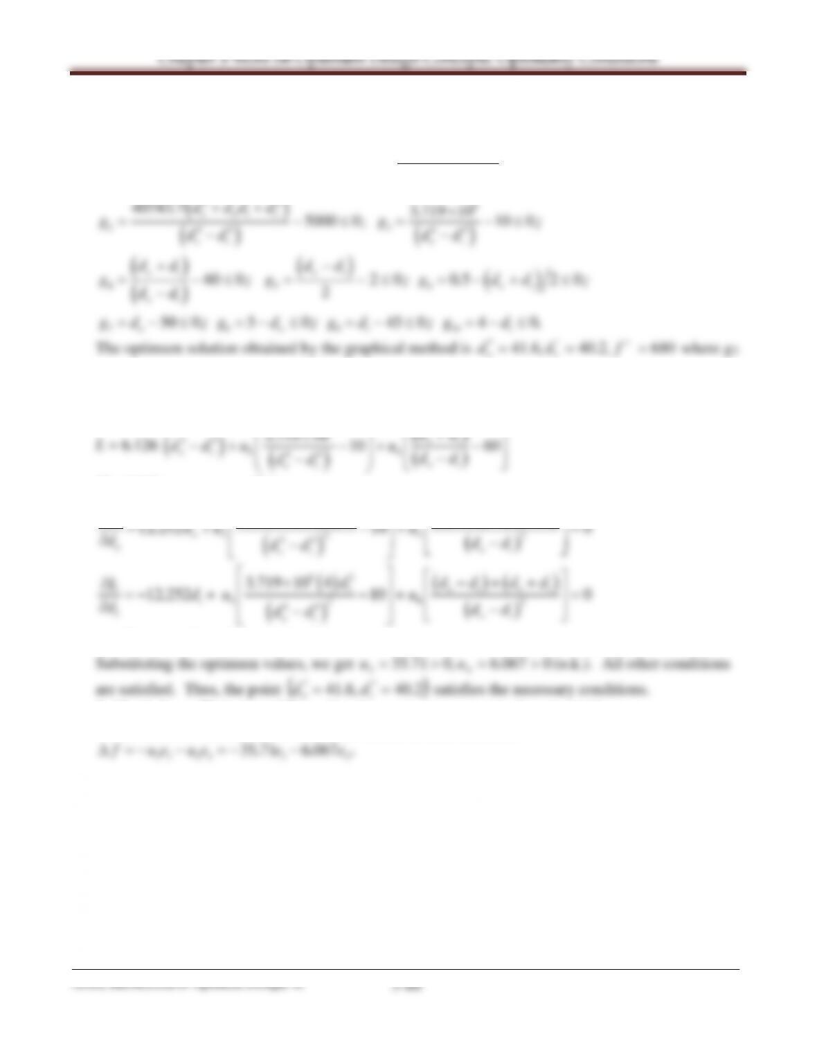
The optimum solution obtained by the graphical method is
∗
== fd
io
,2.40d ,6.41
**
680=
where g3
and g4 are active.
1. Check for necessary conditions.
Since only g3 and g4 are active, we can set u1 = u2 = u5 = u6 = u7 = u8 = u9 = u10 = 0.
( )
6
22
3 719 10 10 60
.
oi
dd
+
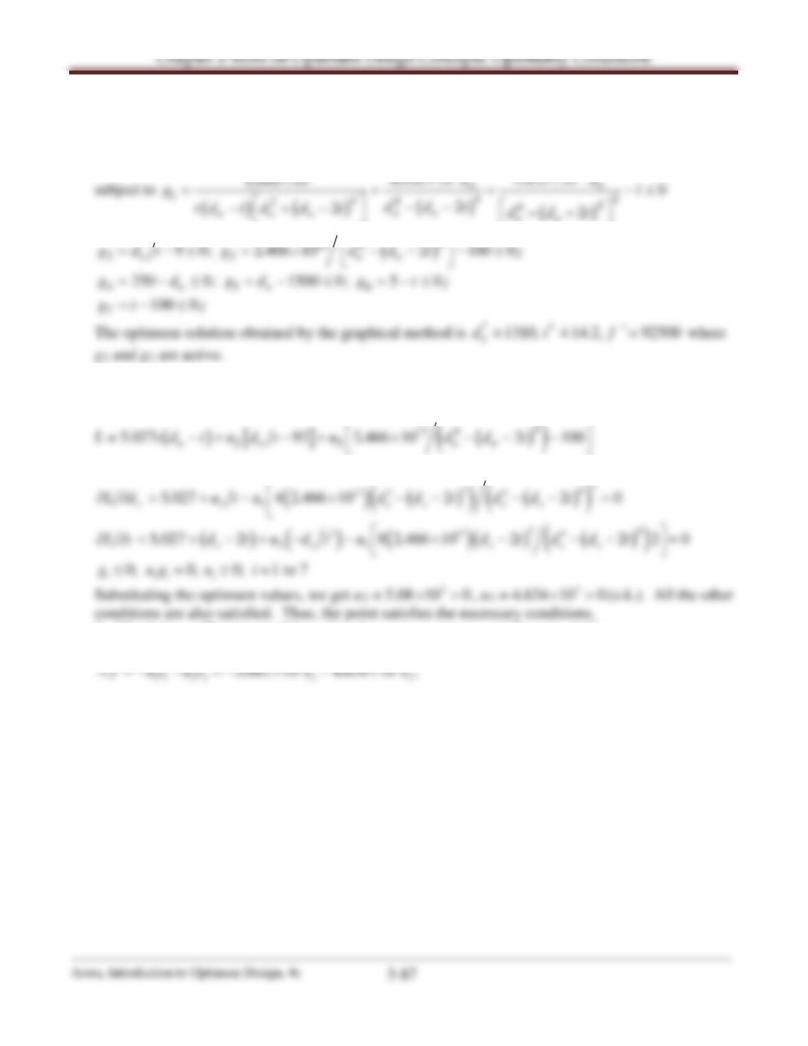
×
5.79________________________________________________________________________________
Referring to the formulation in Exercise 3.53, we have
Minimize f = 5.027t
( )
,
o
dt−
7 17
9
4 098 10 1 435 10
1 688 10 10
oo
dd
××
×
..
.
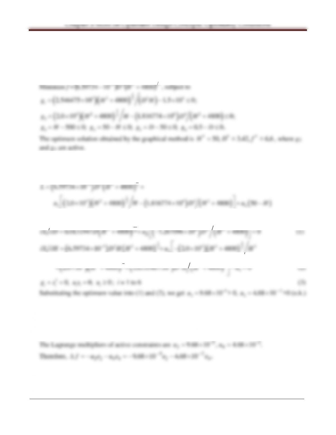
5.80________________________________________________________________________________
The formulation is given in Exercise 3.54.
Optimum solution and check of necessary and sufficient conditions can be found in Exercise 5.48.
Referring to the formulation of Exercise 3.54, we have
21
223
−