Chapter 5 More on Optimum Design Concepts: Optimality Conditions
Referring to the formulation in Exercise 2.1 we have
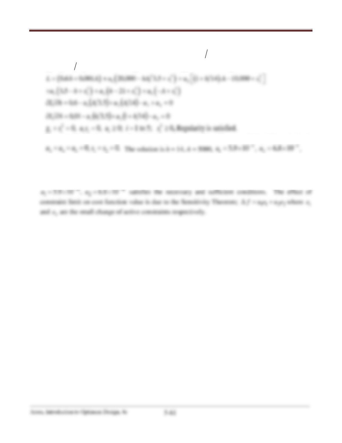
Minimize
1
0 6 0 001 , subject to: g 20,000 3 5 0;f h A hA=+ =−≤.. .
( )
2 3 45
g 1 14 10,000 0; g 3 5 0; g 21 0; g 0hA h h A= + − ≤ = −≤ =− ≤ =−≤.
Arora, Introduction to Optimum Design, 4e
5-62
5.53 ________________________________________________________________________________
Referring to the formulation in Exercises 2.3/4.85, we have
2
12
3 45
20 0; 0; 20 0gR g H gH=−≤ =−≤ =−≤
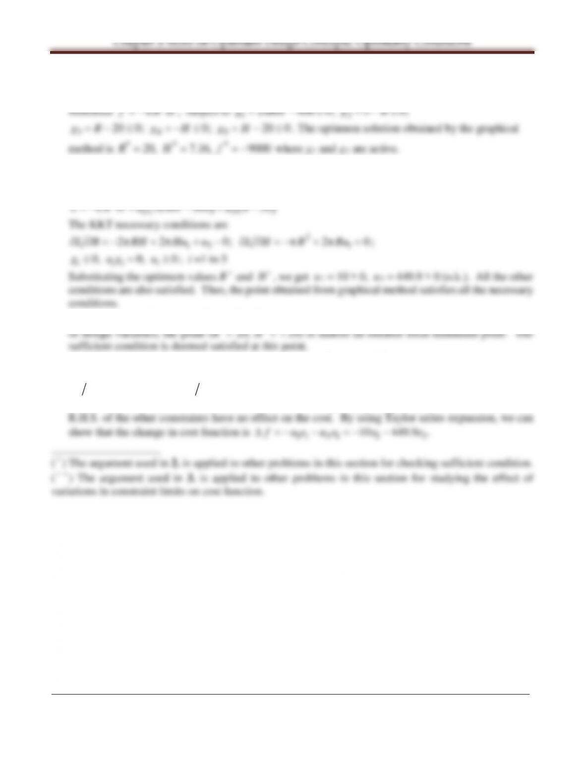
. The optimum solution obtained by the graphical
method is
20, 7.16, 9000RH f
∗∗ ∗
= = = −
where g1 and g3 are active.
1. Check for necessary conditions. Since only g1 and g3 are active, the Lagrange multipliers are
all zero except for u1 and u3. Therefore,
( ) ( )
213
2 900 20L R H u RH u R= −π + π − + −
The KKT necessary conditions are
2
13 1
2 2 0; 2 0L R RH Hu u L H R Ru∂ ∂=−π +π + − ∂ ∂ =−π +π =
;
0, 0, 0
i ii i
g ug u≤=≥
; i =1 to 5
∗
∗
2. Check for sufficient condition (
∗
). Since the number of active constraints is equal to the number
∗
∗
3. Effect of variations in constraint limits on cost function (
∗
∗
). According to the Constraint
Variation Sensitivity Theorem 4.7, we have
11 3 3
10 and 499.9fe u fe u∂∂=− =− ∂∂=− =−
where e1 and e3 are a small variation in the R.H.S. of g1 and g3 respectively. Small variations in
∗
∗
∗
Chapter 5 More on Optimum Design Concepts: Optimality Conditions
5.54 ________________________________________________________________________________
Referring to the formulation in Exercises 2.4/4.86, we have:
2
1. Check for necessary conditions. Since only g1 and g2 are active, set u3 = 0.
( )
( )
2000502 2
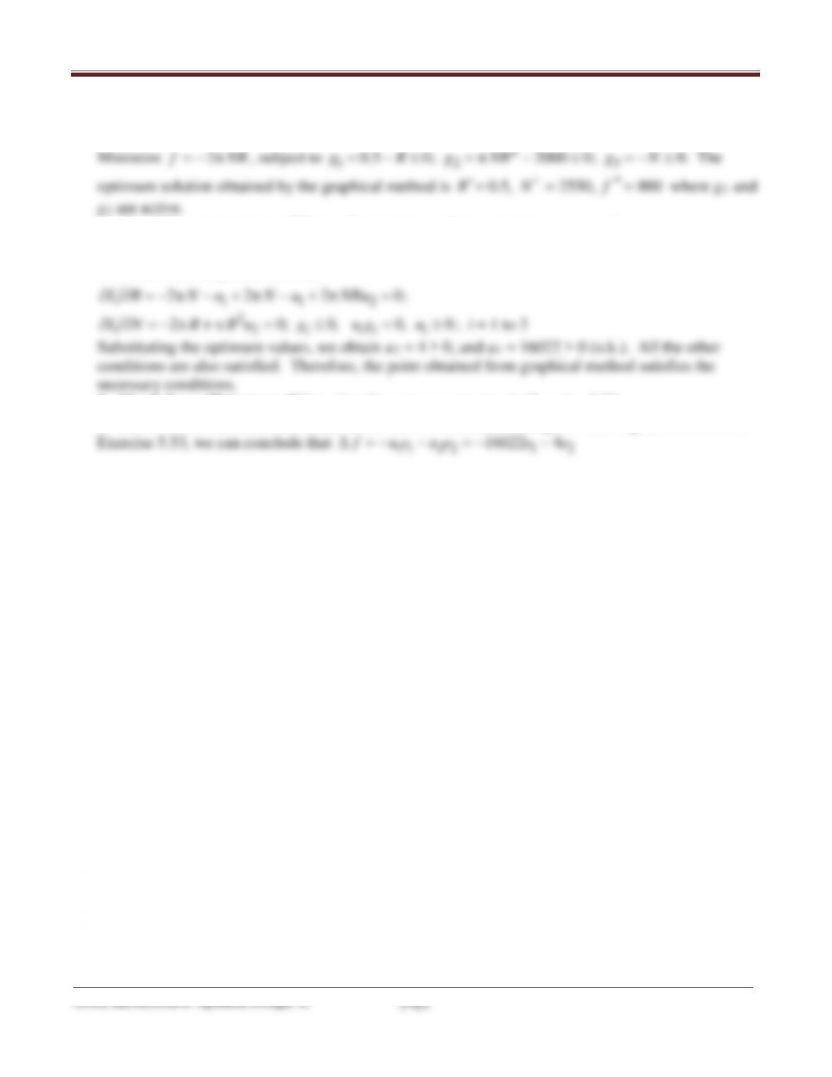
21 −+−+−= NRuR.uNRL
ππ
The KKT necessary conditions are
1 12
2220;LR Nu Nu NRu∂ ∂=−π − +π − +π =
22
2 0; 0, 0, 0
i ii i
L N R R u g ug u∂ ∂ =− π +π = ≤ = ≥
; i = 1 to 3
Substituting the optimum values, we obtain u2 = 4 > 0, and u1 = 16022 > 0 (o.k.). All the other
conditions are also satisfied. Therefore, the point obtained from graphical method satisfies the
necessary conditions.
2. Check for sufficient condition. Use the same argument as in Exercise 5.53.
3. Effect of variations in constraint limits on cost function. Using the same argument as used in
11 2 2 1 2
5.55 ________________________________________________________________________________
Referring to the formulation in Exercises 2.5/4.87, we have:
1. Check for necessary conditions. Since only g3 and g4 are active, set
76521
uuuuu ====
= 0.
( ) ( )
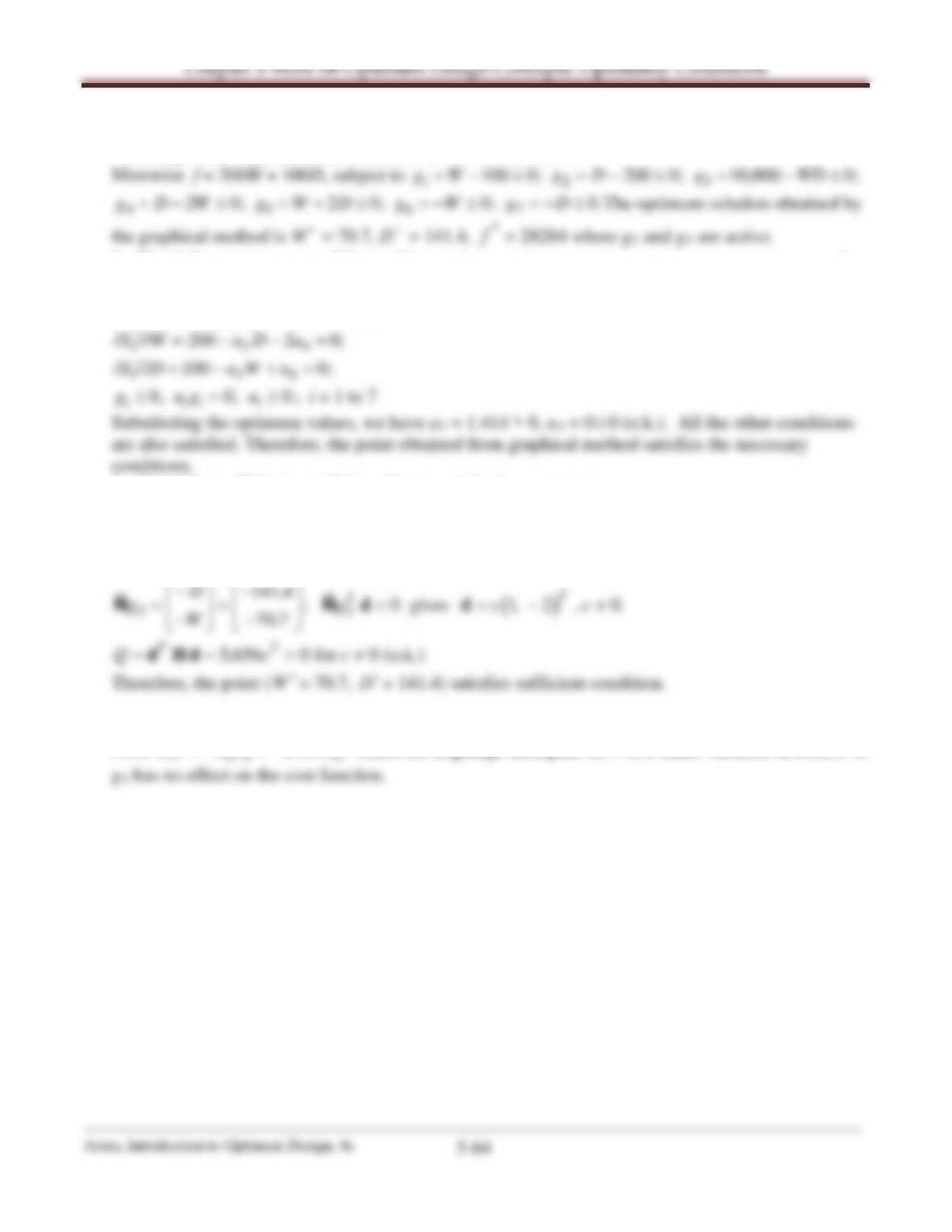
WDuWDuDWL 2000,10100200
43
−+−++=
The KKT necessary conditions are:
34
200 2 0;L W uD u∂∂ = − − =
34
100 0; L D uW u∂∂= − + =
0, 0, 0
i ii i
g ug u≤=≥
; i = 1 to 7
Substituting the optimum values, we have u3 = 1.414 > 0, u4 = 0
≥
0 (o.k.). All the other conditions
are also satisfied. Therefore, the point obtained from graphical method satisfies the necessary
conditions.
2. Check for sufficient condition. Hessian of the Lagrangian is
H =
3
3
00 1.414
01.414 0
u
u
−−
=
−−
Since u4 = 0, we only consider the gradient of g3.
( )
33
2
141 4 ; 0 gives 1, 2 , 0.
70 7
5 656 0 for 0 (o.k.)
T
T
T
D
g g cc
W
Q cc
−−
== = =−≠
−−
= = >≠
.dd
.
d Hd .
ÑÑ
Therefore, the point (
∗
W
= 70.7,
∗
D
= 141.4) satisfies sufficient condition.
3. Effect of variations in constraint limits on cost function. Using the same argument as in Exercise
5.53,
33 3
Δ 1 414f ue e=−=−.
. Since the Lagrange multiplier u4 = 0, a small variation in R.H.S. of
5.56 ________________________________________________________________________________
Referring to the formulation in Exercises 2.9/4.91, we have
22
1. Check for necessary conditions. Since the active constraints are h1 and g1, we can set
5432 uuuu ===
= 0.
( )
( )
22
11
2 600 1 2L r rh v r h u h r=π +π + π − + −
3. Effect of variations in constraint limits on cost function. Using the same argument as used in
1 1 11 1 1
Arora, Introduction to Optimum Design, 4e
5-66
5.57 ________________________________________________________________________________
Referring to the formulation in Exercises 2.10/4.92, we have
Minimize
( ) ( )
bhhbf 15232 +=
, subject to
12
10 0; 18 0gb g h=−≤ =−≤
. The optimum solution
obtained by the graphical method is b
∗
= 10, h
∗
= 18,
f
∗
= 0.545 where g1 and g2 are active.
1. Check for necessary conditions.
( ) ( ) ( ) ( )
181015232
21
−+−++= hububhhbL
The KKT necessary conditions are:
( ) ( )
[ ]
( )
1
2
21532 ubhhhbbhbL ++−=∂∂
= 0;
( ) ( ) ( )
2
2
32 15 2 2 0;
0, 0, 0 1 2
i ii i
L h bh b h b bh u
gugui
∂ ∂= − + + =
≤ = ≥=;,
Substituting the optimum values, we obtain u1 = 0.043 > 0, and u2 = 0.0066 > 0 (o.k.). Thus, the
∗
∗
2. Check for sufficient condition. Use the same argument as in Exercise 5.53.
3. Effect of variations in constraint limits on cost function. Using the same argument as used in
11 2 2 1 2
Chapter 5 More on Optimum Design Concepts: Optimality Conditions
5.58 ________________________________________________________________________________
Referring to the formulation in Exercises 2.12/4.94, we have
2
2
5.59 ________________________________________________________________________________
Referring to the formulation in Exercises 2.14/4.96, we have
22
Chapter 5 More on Optimum Design Concepts: Optimality Conditions
Arora, Introduction to Optimum Design, 4e
5-69
5.61 ________________________________________________________________________________
Formulation is given in Exercise 2.24. Optimum solution and check of necessary and sufficient
conditions can be found in Exercise 5.39.
1. Check for necessary conditions. Since only g1 is active, we can set
765432 uuuuuu =====
= 0
and s1 = 0.
( )
1
1 44086 7957 7 250..L Rt u Rt=+−
.
0.183670. All the other conditions are also satisfied. Thus, the solutions satisfy all of the necessary
conditions.
22 2
11
L fu g= +ÑÑ Ñ
2. Check for sufficient condition.
( ) ( ) ( )
3 22
22 3
2 7957 7 7957 7
0 1 44086 0 1836 7957 7 2 7957 7
1 44086 0
Rt R t
Rt Rt
= +
..
....
.
Substituting 1.44086Rt = 45.9 into
2LÑ
and
1
gÑ
, we have
2
1
2 88 2 88 249 8
2 88 2 88 249 8
Rt t
Lg
tR R
−
= =
−
,
.. .
.. .
ÑÑ
1
0
T
g=dÑ
gives
( )
10
T
c Rt c=−≠d , ,
. Hence,
20
T
QL= =ddÑ
Thus, the sufficient condition is not satisfied. Hence solution is not an isolated local minimum.
The Lagrange multiplier of active constraint is u1 = 0.1836. Therefore,
Δf
=
11 1
0 1836.ue e−=−
.
Chapter 5 More on Optimum Design Concepts: Optimality Conditions
5.62 ________________________________________________________________________________
Optimum solution and check of necessary and sufficient conditions can be found in Exercise 5.41.
Referring to the formulation of Exercise 4.80, we have
5
8
1795 775 2 5 10 0..g Rt= −×≤;
4 10 3
2 3 45
5 10 6 5113 10 0 50 0 0 0.g Rt g Rt g R g t= × − × ≤ = − < =− ≤ =−≤; ; ;
The optimum solution found by the graphical method is
0 0787, 0 00157, 30 56 kg;.. .Rt f
∗∗ ∗
= = =
g
2
3
1. Check for necessary conditions. Since only
2
g
and
3
g
are active, we can set
541 uuu ==
= 0 and
32
ss =
= 0. The KKT necessary conditions are
( )( )
( )
5 10 2
23
2 4662 10 6 5113 10 3 1 0..LR tu Rt u t
∂∂= × + − × + =
(1)
( ) ( )
010511361046622 3
3
310
2
5=−+×−+×=∂∂ tRuR.uR.tL
(2)
2
0 0 0 1 t o 5
i i ii i
g s us u i+= = ≥ =, , ;
(3)
Substituting the optimum value into (1) and (2), we get
4
2
100563
−
×= .u
> 0,
3
u
= 0.3038 > 0 (o.k.).
All of the other constraints in (3) are also satisfied. Thus, the point
( )
001570 ,07870 .t.R == ∗∗
satisfies the necessary conditions.
2. Check for sufficient condition. Since this is the case that the number of active constraints is equal
to the number of design variables, the point is indeed an isolated local minimum.
43
−
5.63 ________________________________________________________________________________
The formulation is given in Exercise 3.24. Optimum solution and check of necessary and sufficient
conditions can be found in Exercise 5.42.
Referring to the formulation of Exercise 4.81, we have
225
42 2 8
1. Check for necessary conditions. Since only g2 and g3 are active, we can set
541 uuu ==
= 0, and s2
and s3 = 0.
( ) ( )
( ) ( )
522 4 1044
23
1 2331 10 5 10 1 62783 10 0 5 50. ..
o i o i oi oi
L RR u RR u RR RR
= × − + ×− × − + + +−
The KKT necessary conditions are
( ) ( )( )
( )
2
5 10 3
23
2 4662 10 1 62783 10 4 0..
o o o ioi
LR R u R u R R R
∂∂ = × + − × + − − =
(1)
( ) ( )( )
( )
2
5 10 3
23
2 4662 10 1 62783 10 4 0..
i i i ooi
LR R u R uR R R
∂∂=− × + × + − =
(2)
20, 0, 0
i i ii i
g s us u+= = ≥
; i = 1 to 5 (3)
Substituting the optimum value into (1) and (2), we get
4
2
100563
−
×= .u
> 0,
3
u
= 0.3055 > 0 (o.k.).
∗∗
2. Check for sufficient condition. Since this is the case that the number of active constraints is
equal to the number of design variables, the point is indeed a local minimum. Sufficient
condition is deemed satisfied at this point.
43
−
Chapter 5 More on Optimum Design Concepts: Optimality Conditions
5.64 ________________________________________________________________________________
The formulation is given in Exercise 4.79. Optimum solution and check of necessary and sufficient
conditions can be found in Exercise 5.43.
Referring to Exercise 4.79, we have
22f DH D=π +π
2
34 5
The optimum solution found by the graphical method is
2
8, 7 98, 300 6 cm..HD f
∗∗ ∗
= = =
where
g1 and g4 are active.
1. Check for necessary conditions. Since only g1 and g4 are active, we can set
532
uuu ==
= 0 and
2. Check for sufficient condition. Since this is the case that the number of active constraints is equal
to the number of design variables, the point is indeed local minimum point.
5.65 ________________________________________________________________________________
The formulation is given in Exercise 3.28. Optimum solution and check of necessary and sufficient
conditions can be found in Exercise 5.40.
Rewrite the formulation of Exercise 3.28, we have
2
2
1. Check for necessary conditions. Since only g1 and g2 are active, we can set
543
uuu ==
= 0 and
21 ss =
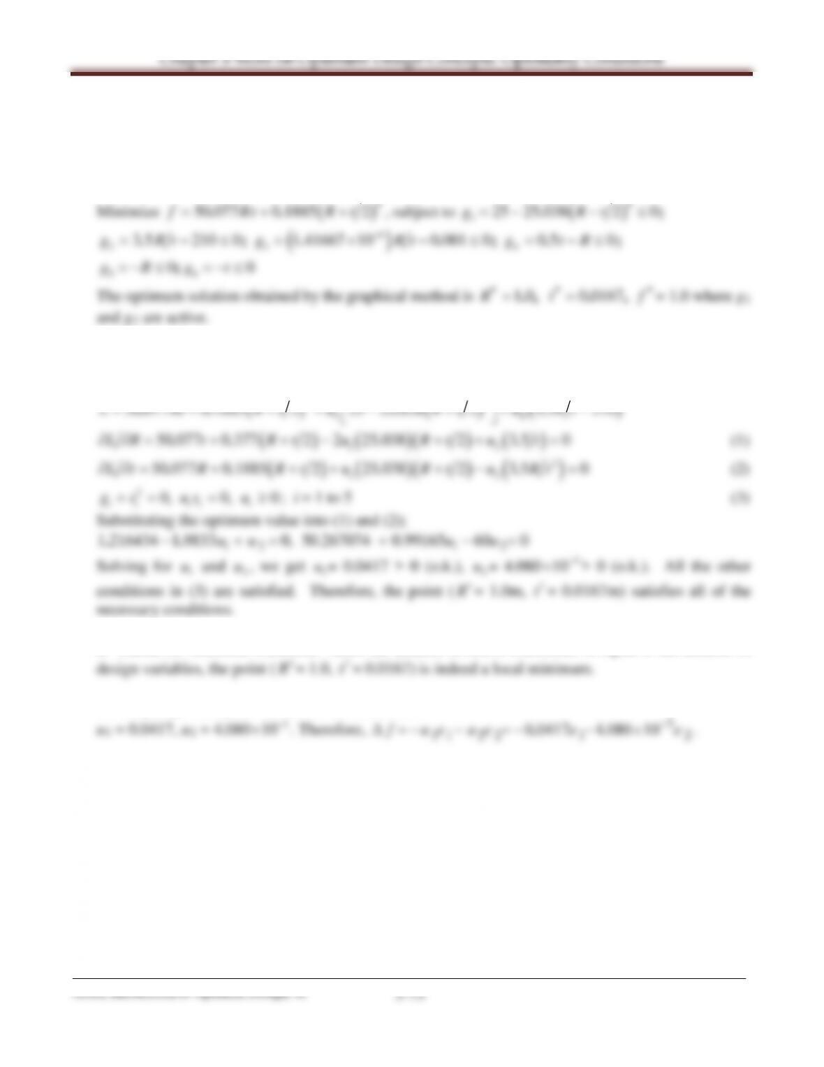
= 0.
( ) ( ) ( )
22
12
50 077 0 1885 2 25 25 038 2 3 5 210.. . .L Rt Rt u Rt u Rt
=+++−++−
( ) ( )( ) ( )
12
50 077 0 377 2 2 25 038 2 3 5 0LR t Rt u Rt u t∂∂= + +− ++ =.. . .
(1)
( ) ( )( )
( )
2
12
50 077 0 1885 2 25 038 2 3 5 0Lt R Rt u Rt u Rt∂∂= + ++ +− =.. . .
(2)
20, 0, 0
i i ii i
g s us u+= = ≥
; i = 1 to 5 (3)
Substituting the optimum value into (1) and (2);
12 1 2
1 216434 1 9833 0, 50.267074 0.99165 60 0uu u u− += + − =..
Solving for
1
u
and
2
u
, we get
1
u
= 0.0417 > 0 (o.k.),
2
u
= 4.080
3
10−
×
> 0 (o.k.). All the other
conditions in (3) are satisfied. Therefore, the point ( ∗
R
= 1.0m,
∗
t
= 0.0167m) satisfies all of the
necessary conditions.
2. Check for sufficient condition. Since the number of active constraints is equal to the number of
∗
∗
The Lagrange multipliers of active constraints are
10−
×
3
3
−
( )( )
( )
25
42
3 12
4 17246 10 3 1 0
.
.u xx
+− × − =
5.66 ________________________________________________________________________________
The formulation is given in Exercise 3.34*. Optimum solution and check of necessary and sufficient
conditions can be found in Exercise 5.45.
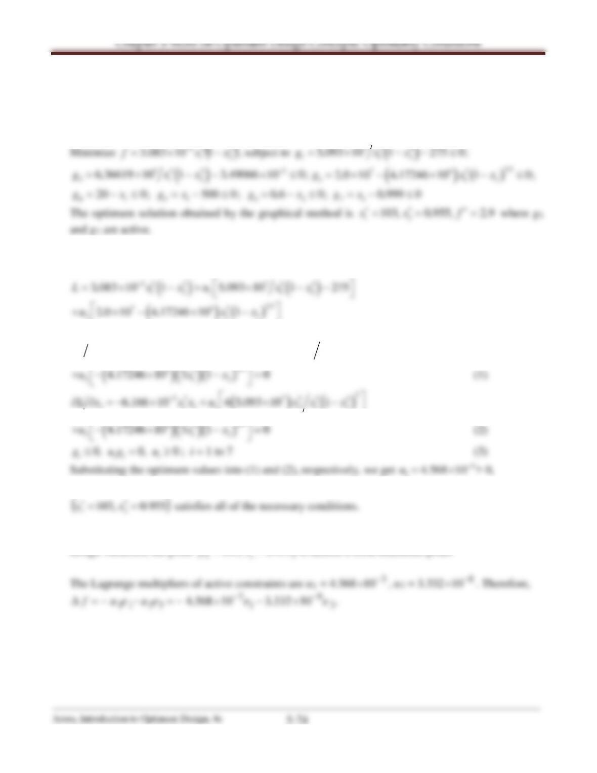
Rewriting the formulation of Exercise 3.34, we have
2
2
3
−
73 4
1. Check for necessary conditions. Since only g1 and g3 are active, we can set
u2 = u4 = u5 = u6 = u7 = 0.
( ) ( )
32 2 7 3 4
1 21 1 2
3 083 10 1 5 093 10 1 275..L x xu x x
−
= × −+ × −−
25
7 43
3 12
.
The KKT necessary conditions are
( ) ( ) ( )
3 2 74 4
1 1 21 1 2
6 166 10 1 3 5 093 10 1..Lx x x u x x
−
∂∂= × − + − × −
( )( )
( )
25
42
3 12
4 17246 10 3 1 0
.
.u xx
+− × − =
(1)
2
32 7 3 3 4
−