4
gÑ
Case 15.
0 ,0
3214
==== sssu
; gives no candidate point.
Case 16.
0
4321
==== ssss
; gives no candidate point.
Check for regularity: For cases 1, 2, 3, 4 and 5, there is only one active constraint, so regularity is
satisfied. For case 6,
( ) ( )
34
g 1, 0 , g 0, 1=−=−ÑÑ
. Since
3
gÑ
and
4
gÑ
are linearly independent,
2
gÑ
gÑ
Arora, Introduction to Optimum Design, 4e
5-42
5.36 ________________________________________________________________________________
Solve the following problem graphically. Check necessary and sufficient conditions for candidate
local minimum points and verify them on the graph for the problem.
Maximize (,)= ( − 8)2+ ( − 8)2
subject to + ≤ 10
≥ 0
≤ 0
Solution
Minimize
( ) ( ) ( )
22
1
, 8 8 ; subject to g 10 0;f rt r t r t=− − − − = +− ≤
23
g 0; g 0;rt= ≤ =−≤
( ) ( )
()
( ) ( )
( )
( ) ( )
22 22
1 12 2
2
33
13 12
8 8 10
2 8 0; 2 8 0;
L r t urt s u t s
urs
Lr r u u Lt t u u
=− − − − + + − + + −+
++
∂∂=− − + + = ∂∂=− − + + =
2 22
1 23
10 0; 0; 0;rt s ts rs+−+= −+= +=
;0 ;0 ≥= iii usu
i = 1 to 3 (there are 8 cases).
Case 1.
123
0uuu= = =
; no candidate minimum.
Case 5.
1 23
0, 0u ss= = =
; no candidate minimum.
Case 7.
3 12
0, 0u ss= = =
; no candidate minimum.
Refer to Exercise 4.77/4.130. There are no points that satisfy the KKT necessary conditions.
Chapter 5 More on Optimum Design Concepts: Optimality Conditions
5.37 ________________________________________________________________________________
Solve the following problem graphically. Check necessary and sufficient conditions for candidate
local minimum points and verify them on the graph for the problem.
Maximize (,)= ( − 3)2+ ( − 2)2
subject to 10 ≥ +
≥ 5
, ≥ 0
Solution
Minimize
( ) ( )
( )
22
1
, 3 2 ; subject to g 10 0;f rt r t r t=− − − − = +− ≤
2 34
g 5 0; g 0; g 0;t rt=−+ ≤ =− ≤ =−≤
( ) ( )
()
( ) ( )
( ) ( )
( ) ( )
22 22
1 12 2
22
3 34 4
13 124
3 2 10 5
2 3 0; 2 2 0;
L r t urt s u t s
u rs u ts
Lr r u u Lt t u u u
=− − − − + + − + + −+ +
+ −+ + −+
∂∂=− − + − = ∂∂=− − + − − =
2 2 22
1 2 34
10 0; t+5 0; 0; 0;rt s s rs ts+−+= − += −+= −+=
;0 ;0 ≥= iii usu
i = 1 to 4 (there are 16 cases).
Case 1.
1234
0;uu uu= = = =
gives no candidate point.
Case 14.
0 ,0
4213
==== sssu
; gives no candidate point.
0 ,0
3214
Case 16.
0
4321
==== ssss
; gives no candidate point.
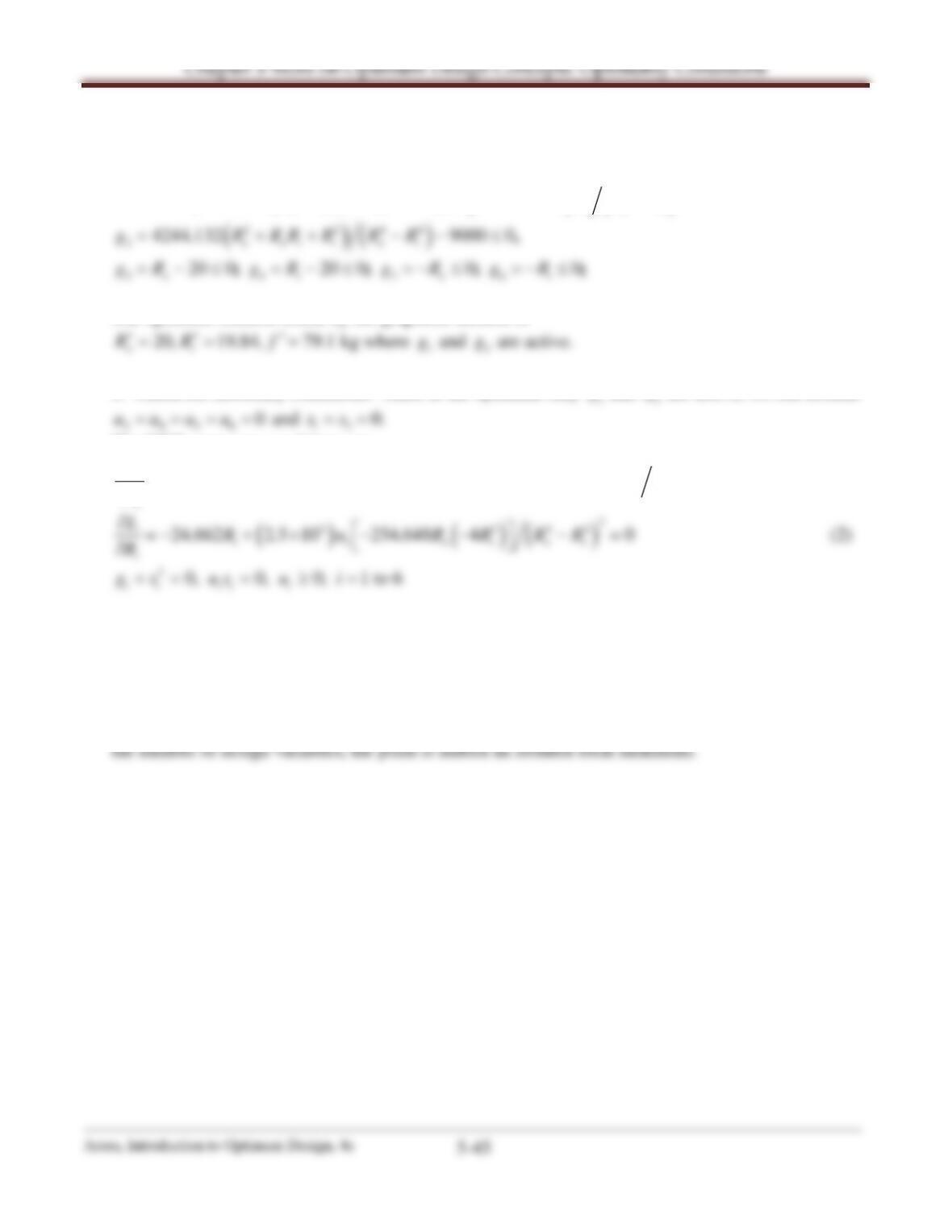
Check for regularity: For cases 4, there is only one active constraint, so regularity is satisfied. For
5.38 ________________________________________________________________________________
Rewrite the formulation of Exercise 2.23, the problem is written in the standard form as (note that
some of the data used here is different from that used in Exercise 2.23):
Minimize
( )
22
33112
io
RR.f −=
, subject to
( ) ( )
6 44 4
1
6 3662 10 2 5 10 0..
oo i
g RRR= × − −×≤
( ) ( )
2 2 44
2
46
4244 132 9000 0
20 0 20 0 0 0
.o oi i o i
3o i 5 o i
g R RR R R R
gR gR g R g R
= + + −− ≤
=−≤ =−≤ =−≤ =−≤
,
; ; ; ;
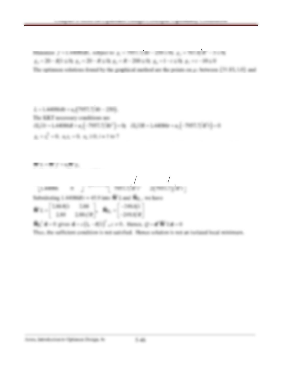
The optimum solution found by the graphical method is
∗∗∗ == f.RR io ,8419 ,20
5.39 ________________________________________________________________________________
Rewriting the formulation of Exercise 2.24, we have
2
( )
25.23 1 26,.
, where
∗
f
= 45.9 and g1 is active.
1. Check for necessary conditions. Since only g1 is active, we can set
765432 uuuuuu =====
= 0
and s1 = 0.
( )
1
1 44086 7957 7 250..L Rt u Rt=+−
.
The KKT necessary conditions are
( ) ( )
22
11
1 44086 7957 7 0 1 44086 7957 7 0. . ..Lt Ru Rt LR tu Rt∂∂= + − = ∂∂= + − =;
2
0, 0,
i i ii i
g s us u+= = ≥
0; i = 1 to 7
Using the relation, 1.44086Rt = 45.9 at optimum solutions, and either equation, we can obtain u1 =
0.183670. All the other conditions are also satisfied. Thus, the solutions satisfy all of the necessary
conditions.
22 2
11
L fu g= +ÑÑ Ñ
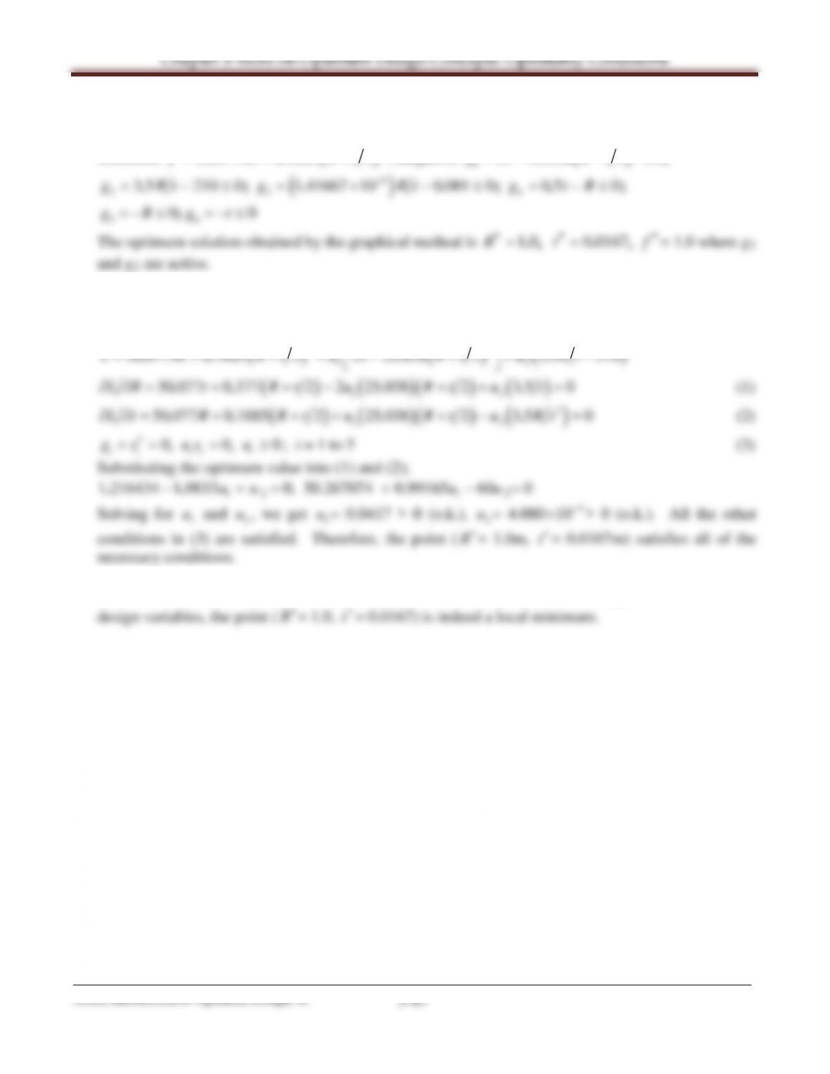
2. Check for sufficient condition.
( ) ( ) ( )
3 22
22 3
2 7957 7 7957 7
0 1 44086 0 1836 7957 7 2 7957 7
1 44086 0
Rt R t
Rt Rt
= +
..
....
.
2LÑ
5.40________________________________________________________________________________
Rewrite the formulation of Exercise 3.28, we have
Minimize
( )
2
50 077 0 1885 2f Rt R t=++..
, subject to
( )
2
1
25 25 038 2 0.g Rt=− −≤;
( )
5
23 4
3 5 210 0 1 41667 10 0 001 0 0 5 0g Rt g Rt g t R
−
= − ≤ = × − ≤ = −≤; ; ;. . ..
56
00gRgt=− ≤ =−≤;
The optimum solution obtained by the graphical method is
1 0 0 0167Rt f
∗∗ ∗
= =., . ,
= 1.0 where g1
and g2 are active.
1. Check for necessary conditions. Since only g1 and g2 are active, we can set
543
uuu ==
= 0 and
21 ss =
= 0.
( ) ( ) ( )
22
12
50 077 0 1885 2 25 25 038 2 3 5 210.. . .L Rt Rt u Rt u Rt
=+++−++−
( ) ( )( ) ( )
12
50 077 0 377 2 2 25 038 2 3 5 0LR t Rt u Rt u t∂∂= + +− ++ =.. . .
(1)
( ) ( )( )
( )
2
12
50 077 0 1885 2 25 038 2 3 5 0Lt R Rt u Rt u Rt∂∂= + ++ +− =.. . .
(2)
20, 0, 0
i i ii i
g s us u+= = ≥
; i = 1 to 5 (3)
Substituting the optimum value into (1) and (2);
12 1 2
1 216434 1 9833 0, 50.267074 0.99165 60 0uu u u− += + − =..
Solving for
1
u
and
2
u
, we get
1
u
= 0.0417 > 0 (o.k.),
2
u
= 4.080
3
10−
×
> 0 (o.k.). All the other
conditions in (3) are satisfied. Therefore, the point (
∗
R
= 1.0m,
∗
t
= 0.0167m) satisfies all of the
necessary conditions.
2. Check for sufficient condition. Since the number of active constraints is equal to the number of
R
t
∗
∗
5.41 ________________________________________________________________________________
Referring to the formulation of Exercise 4.80, we have
5
8
1795 775 2 5 10 0..g Rt= −×≤;
4 10 3
2 3 45
5 10 6 5113 10 0 50 0 0 0.g Rt g Rt g R g t= × − × ≤ = − < =− ≤ =−≤; ; ;
The optimum solution found by the graphical method is
0 0787, 0 00157, 30 56 kg;.. .Rt f
∗∗ ∗
= = =
g
2
3
1. Check for necessary conditions. Since only
2
g
and
3
g
are active, we can set
541 uuu ==
= 0 and
32
ss =
= 0. The KKT necessary conditions are
( )( )
( )
5 10 2
23
2 4662 10 6 5113 10 3 1 0..LR tu Rt u t
∂∂= × + − × + =
(1)
( ) ( )
010511361046622 3
3
310
2
5=−+×−+×=∂∂ tRuR.uR.tL
(2)
2
0 0 0 1 t o 5
i i ii i
g s us u i+= = ≥ =, , ;
(3)
Substituting the optimum value into (1) and (2), we get
4
2
100563
−
×= .u
> 0,
3
u
= 0.3038 > 0 (o.k.).
All of the other constraints in (3) are also satisfied. Thus, the point
( )
001570 ,07870 .t.R == ∗∗
satisfies the necessary conditions.
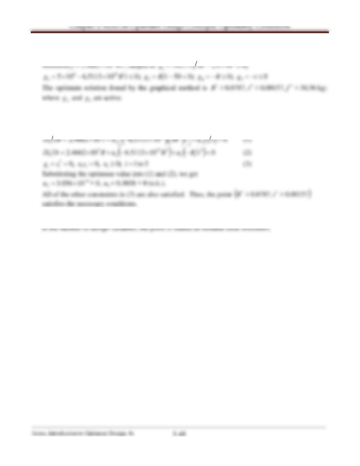
2. Check for sufficient condition. Since this is the case that the number of active constraints is equal
Chapter 5 More on Optimum Design Concepts: Optimality Conditions
5.42 ________________________________________________________________________________
Referring to the formulation of Exercise 4.81, we have
225
42 2 8
5.43________________________________________________________________________________
Referring to Exercise 4.79, we have
22f DH D=π +π
2
12
34 5
8 0; 8 0; 18 0gD g H gH= −≤ =− ≤ = − ≤
The optimum solution found by the graphical method is
2
8, 7 98, 300 6 cm..HD f
∗∗ ∗
= = =
where
g1 and g4 are active.
1. Check for necessary conditions. Since only g1 and g4 are active, we can set
532
uuu ==
= 0 and
s1 = s4 = 0.
( )
( )
22
14
2 400 4 8L DH D u D H u H=π +π + −π + −
The KKT necessary conditions are
( )
( )
2
1 14
2 0; 4 0LD H Du DH LH Du D u∂ ∂ =π + π + −π = ∂ ∂ =π + −π − =
20, 0, 0
i i ii i
g s us u+= = ≥
; i = 1 to 5
Substituting the optimum value into equations, we get u1 = 0.5 > 0, u4 = 0.063 > 0 (o.k.). All the
2. Check for sufficient condition. Since this is the case that the number of active constraints is equal
to the number of design variables, the point is indeed local minimum point.
5.44 ________________________________________________________________________________
Rewriting the formulation of Exercise 4.83, we have
1. Check for necessary conditions.
( ) ( ) ( )
h.uA.hA.u.hA,uA.h.L −+−++−++= 53000,10532505300020001060 321
( )
Auhu 54 21 −−+
The KKT necessary conditions are
( ) ( )
015325053010 521 =−++−+=∂∂ u.h.u.hu.AL
(1)
( ) ( )
0532505360 4321 =+−+−+=∂∂ uu.A.u.Au.hL
(2)
0, 0, 0
i ii i
g ug u≤=≥
; i =1 to 5 (3)
543
uuu ==
2. Check for sufficient condition. Since the number of constraints active at the candidate point and
25
.
5.45 ________________________________________________________________________________
Rewriting the formulation of Exercise 3.34, we have
Minimize
( )
2
2
2
1
3
1100833 xx.f −×=
−
, subject to
( )
73 4
1 12
5 093 10 1 275 0;.g xx= × −− ≤
( )
54 4 2
2 12
6 36619 10 1 3 49066 10 0;..g xx
−
= × −− × ≤
( )
( )
25
7 43
3 12
2 0 10 4 17246 10 1 0;
.
..g xx=×− × − ≤
4 1 51
20 0; 500 0;g x gx= −≤ =− ≤
6 2 72
0 6 0; 0 999 0..g x gx= −≤ =− ≤
The optimum solution obtained by the graphical method is
12
103, 0 955, 2 9..xx f
∗∗ ∗
= = =
where g1
and g3 are active.
1. Check for necessary conditions. Since only g1 and g3 are active, we can set u2 = u4 = u5 = u6 = u7
= 0.
( ) ( )
32 2 7 3 4
1 21 1 2
3 083 10 1 5 093 10 1 275..L x xu x x
−
= × −+ × −−
( )
( )
25
7 43
3 12
2 0 10 4 17246 10 1
.
..u xx
+ ×− × −
The KKT necessary conditions are
3 2 74 4
1 1 21 1 2
−
25
42
.
5.46 ________________________________________________________________________________
Rewriting the formulation of Exercise 3.35, we have
Minimize
( )
223
100833
io
dd.f −×=
−
, subject to
( ) ( )
7 44
15 093 10 275 0;.oo i
g ddd= × −−≤
( ) ( )
5 44 2
2
6 3662 10 3 49066 10 0;..
oi
g dd
−
= × −− × ≤
( )
( )
25
7 43
34
2 0 10 4 17246 10 1 0; 20 0;
.
..
o io o
g d dd g d= × − × − ≤ =−≤
56 7
500 0; 0 6 0; 0 999 0;..
o io io
g d g dd g dd=−≤ =− ≤ = − ≤
1
g
∗∗∗
3
1. Check for necessary conditions. Since only
1
g
and
3
g
are active, we can set
76542
uuuuu ====
= 0.
( ) ( ) ( )
322 7 22
1
3.083 10 5.093 10 275
oi ooi
L dd u ddd
−
= × −+ × −−
( )
( )
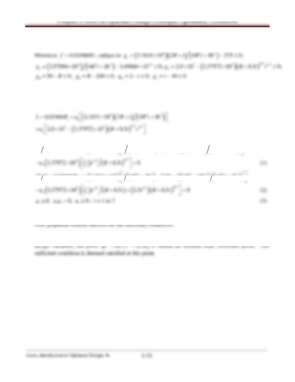
2.5
7 43
3
2.0 10 4.17246 10 1
o io
u d dd
+ ×− × −
5.47 ________________________________________________________________________________
Rewriting the formulation of Exercise 3.36, we have
6 33
4
5 67
The optimum solution obtained by the graphical method is
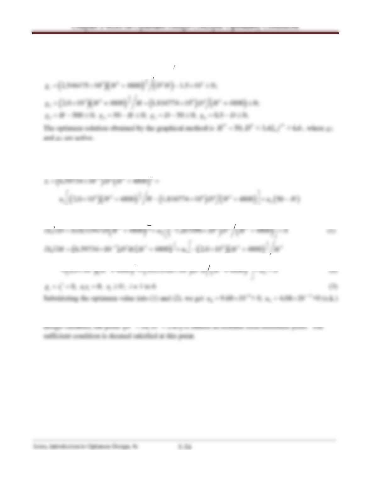
92 ,342 ,350 .f.t.R === ∗∗∗
where g1
and g3 are active.
1. Check for necessary conditions. Since only g1 and g3 are active, we can set
24567
0.uuuuu= = = = =
( )
( )
( )
6 33
1
0 02466 3 1831 10 2 4..
t
L R u R t R t Rt
= + ×+ +
( )
( )
05
7 5 25
3
2 0 10 3 37972 10 0 5
..
.. .u R tt
+ ×− × +
The KKT necessary conditions are
( ) ( )
( )
( ) ( )
2
6 33 23 33
1
0 02466 3 1831 10 2 4 2 12 4..L R t u R t Rt R t R t R t Rt
∂∂= + × + − + + +
( )
( )
( )
05
5 25
1
32
3 37972 10 0 5 0
.
.
..u tR t
− × +=
(1)
( ) ( )
( )
( ) ( )
2
6 33 3 2 33
1
0 02466 3 1831 10 1 4 2 4 3 4..L t R u R t Rt R t R Rt R t Rt
∂ ∂= + × + − + + +
( )
( )
( )
( )
( )
05
5 25 15
1
34
3 37972 10 0 5 2 5 0 5 0u tRt tRt
− × ++ + =
.
..
. .. .
(2)
0, 0, 0
i ii i
g ug u≤=≥
; i = 1 to 7 (3)
Substituting the optimum value into (1) and (2) respectively, we obtain u1 =
3
106434
−
×.
> 0, u3 =
8
102403
−
×.
> 0 (o.k.). All the other conditions in (3) are also satisfied. Therefore, the point obtained
2. Check for sufficient condition. Since the number of active constraints is equal to the number of
∗∗
5.48 ________________________________________________________________________________
Referring to the formulation of Exercise 3.54, we have
Minimize f =
( ) ( )
21
223
480010597346 +−
−
HD.
, subject to
( )( ) ( )
( )( ) ( ) ( )
1
42 2 4
2
1
1
4 2 64 2
2
2
2 546475 10 4800 1 5 10 0;
2 0 10 4800 1 816774 10 4800 0;
..
..
g H DH
g H H DH
= × + −× ≤
=× + − × +≤
3 4 56
500 0; 50 0; 50 0; 0 5 0..gH g H gD g D=− ≤ = −≤ =− ≤ = −≤
The optimum solution obtained by the graphical method is
50, 3 42, 6 6HD f
∗∗ ∗
= = =
..
, where g2
and g4 are active.
1. Check for necessary conditions. Since only g2 and g4 are active, we can set
6531 uuuu ===
= 0
and
0
42
== ss
.
( ) ( )
( )( ) ( ) ( )
( )
1
32 2 2
1
4 2 64 2
2
24
6 59734 10 4800
2 0 10 4800 1 816774 10 4800 50
.
..
L DH
u H H DH u H
−
= × ++
× + − × + +−
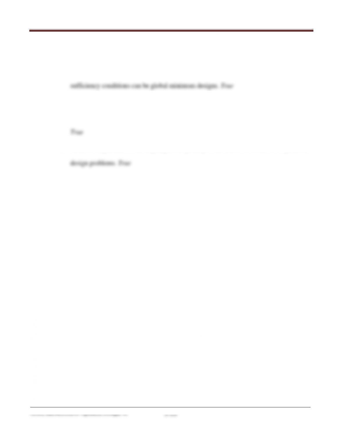
The KKT necessary conditions are
( ) ( ) ( )
1
2 63 2
22
0 0131947 4800 7 267096 10 4800 0..L D DH u D H
∂∂= + + − × + =
(1)
11
32 2 4 2 2
22
−
Chapter 5 More on Optimum Design Concepts: Optimality Conditions
5.49 ________________________________________________________________________________
Answer True or False.
1. Candidate minimum points for a constrained problem that do not satisfy second-order
2. Lagrange multipliers may be used to calculate the sensitivity coefficient for the cost
function with respect to the right side parameters even if Theorem 4.7 cannot be used.
3. Relative magnitudes of the Lagrange multipliers provide useful information for practical
5.50 ________________________________________________________________________________
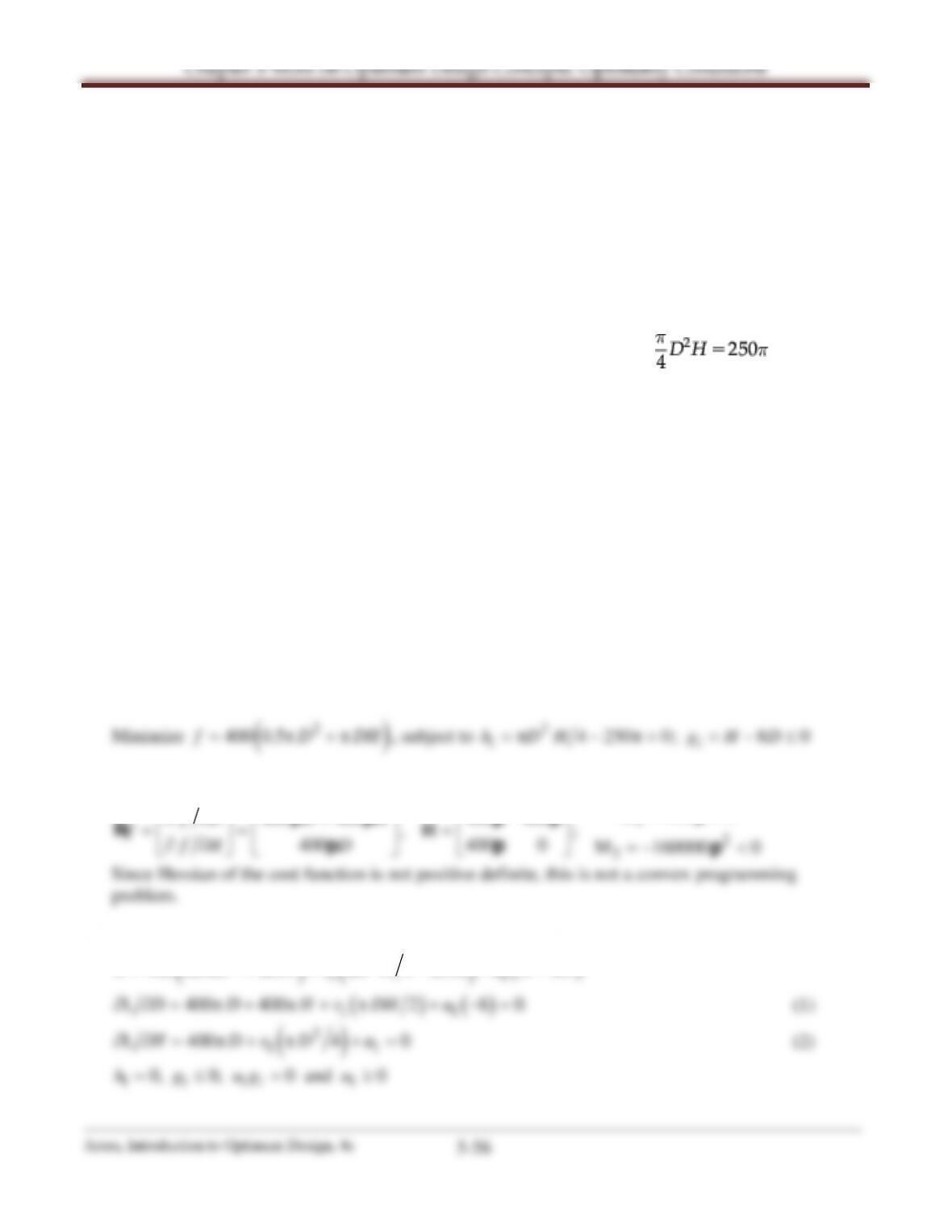
A circular tank that is closed at both ends is to be fabricated to have a volume of 250π m3. The
fabrication cost is found to be proportional to the surface area of the sheet metal needed for fabrication
of the tank and is $400/m2. The tank is to be housed in a shed with a sloping roof which limits the height
of the tank by the relation H≤8D, where H is the height and D is the diameter of the tank. The problem is
formulated as minimize f(D,H)=400(0.5πD2+πDH) subject to the constraints , and H≤8D.
Ignore any other constraints.
1. Check for convexity of the problem.
2. Write KKT necessary conditions.
3. Solve KKT necessary conditions for local minimum points. Check sufficient conditions
and verify the conditions graphically.
4. What will be the change in cost if the volume requirement is changed to 255π m3 in place
of 250π m3?
11
1. Check for convexity of the problem.
1
2
2
M 400 0
400 400 400 400
, ;
400 400 0 M 160000 0
fD D H
ffH D
= >
∂∂ +
= = =
∂∂ =−<
Hp
p p pp
Ñpp p
Since Hessian of the cost function is not positive definite, this is not a convex programming
problem.
2. Write Kuhn-Tucker necessary conditions.
( ) ( )
( )
22
11
L 400 0 5 4 250 8D DH v D H u H D= π +π + π − π + −.
( ) ( )
11
L 400 400 2 8 0D D H v DH u∂∂= π+ π + π + − =
(1)
( )
2
11
L 400 4 0H Dv D u∂∂= π+ π + =
(2)
1 1 11 1
0, 0, 0 and 0h g ug u=≤= ≥
3. Solve the KKT conditions.
Case 2. u1 = 0. Solving the equations, we obtain D = H = 10,
160
1
−=v
.
4. Change in cost.
Applying the constraint variation sensitivity theorem, we get the cost increase as
( )
11
Δ 160 225 250 800f ue=−= − =pp p
5.51 ________________________________________________________________________________
A symmetric (area of member 1 is the same as area of member 3) three-bar truss problem is
described in Section 2.10.
1. Formulate the minimum mass design problem treating A1 and A2 as design variables.
3. Write KKT necessary conditions for the problem.
4. Solve the optimum design problem using the data: P=50 kN, θ=30°, ρ=7800 kg/m3,
5. What will be the effect on the cost function if σa is increased to 152 MPa?
1. Referring to Section 2.10, the design problem is formulated as
Minimize
( )
12
22f l AA= +r
, subject to
( )
1 1 12 1 2
2 22 0
a
g s As A A= + + −σ ≤
( )
2 21 2 3 1 4 2
2 2 0, 0, 0
a
g sA A g A g A= + −σ ≤ =− ≤ =− ≤
3. Write Kuhn-Tucker necessary conditions.
( ) ( ) ( )
1211 12 1 2 2 21 2
22 2 2 2 2 2
aa
L l A A us A s A A u s A A
=ρ + + + + −σ + + −σ
( ) ( )
314 2
uAuA+− + −
( ) ( )
22 2
1 1112 12 2212 3
22 2 2 2 2 2 0LA lusAs AA u sAA u
∂∂=ρ+−− ++−+−=
( ) ( )
22
2 121 2 2 2 1 2 4
2 22 0LA lusA A u sA A u
∂∂=ρ+−++−+−=
1, 2, 3, 4
0, 0, 0;
i ii i
g ug u i≤ = ≥=
4. Solve the design problem. Use Newton, meter and kilogram as units for force, length and mass
respectively.
4
a
8
l = 1 m,
44
12
cos 4.330127 10 N, sin 2.5 10 NsP s P==×==×qq
Substituting the above values we have:
Minimize
( )
21
3
221087 AA.f +×=
Chapter 5 More on Optimum Design Concepts: Optimality Conditions
subject to
()
44 8
11 2
1
4.330127 10 2 2.5 10 2 2 1.5 10 0g A AA= × +× + −× ≤
( )
( )
48
2 12 3 4
12
2 2.5 10 2 1.5 10 0; 0; 0g A A gA gA= × + −× ≤ =−≤ =− ≤
The KKT conditions become
2
3 42 4
Chapter 5 More on Optimum Design Concepts: Optimality Conditions
5.52 ________________________________________________________________________________
A 100 ×100m lot is available to construct a multistory office building. At least 20,000 m2 total
floor space is needed. According to a zoning ordinance, the maximum height of the building can
be only 21m, and the area for parking outside the building must be at least 25 percent of the floor
area. It has been decided to fix the height of each story at 3.5m. The cost of the building in millions
of dollars is estimated at 0.6 h +0.001 A, where A is the cross-sectional area of the building per
floor and h is the height of the building. Formulate the minimum cost design problem.
Solution