Chapter 4 Optimum Design Concepts
4.136_______________________________________________________________________________
Check for convexity of the following function. If the function is not convex everywhere, than
determine the domain (feasible set S)over which the function is convex.
(1,2)=1
2+ 412+2
2+ 3
Solution
( )
34 , 2
221
2
121 +++= xxxxxxf
12
12
12
24 24
, ; 2 0; 12 0
42 42
xx
f MM
xx
+
∇= = = > =− >
+
H.
Function f is not convex since the Hessian is indefinite. We cannot find a domain over which
function f is convex because the Hessian is always indefinite.
4.137_______________________________________________________________________________
Check for convexity of the following function. If the function is not convex everywhere, than
determine the domain (feasible set S)over which the function is convex.
(1,2)=1
3+1212
2+ 22
2+ 51
2+ 32
Solution
( )
2
2
1
2
2
2
21
3
121 35212 , xxxxxxxxf ++++=
12
22
1 1 2 1 2 12 2
21
6 10 24
3 12 10 ; 24 4 3; 24 24 4
xx
fx x x x fx xx x xx
+
∂∂= + + ∂∂ = + + =
+
H
Since Hessian is not always positive semidefinite, the function is not convex everywhere. To find
the domain over which the function is convex, we need to impose the following conditions:
( )
11
6 10 0 1Mx= +≥
( )( ) ( ) ( )
2
21 1 2
6 10 24 4 24 0 2Mx x x= + +− ≥
From (1),
35
1
−≥x
.
From (2),
057640264144 2
21
2
1≥−++ xxx
, or
( )
( )
22
2 11
1 576 144 264 144 40 144x xx
≤ ++
/ / /,
( )
( )
1
22
1 4 11 12 9 16
2
or x x≤ +−
/ //,
or
( )
22
12
11 12 4 9 16 0xx+ −− ≥/.
4.138_______________________________________________________________________________
Check for convexity of the following function. If the function is not convex everywhere, than
determine the domain (feasible set S)over which the function is convex.
(1,2)= 51−(116
⁄)1
22
2+2
241
⁄
Solution
( ) ( )
,41615 , 1
2
2
2
2
2
1121 xxxxxxxf +−=
2 22 2 23 2
12 21 2 21 12 21
2 22
1 2 2 1 12 2 1 1 1
5 84 82 42
;
8 2 4 2 8 12
xx xx x xx xx xx
fx x x x xx x x x x
− − −+ − −
= =
− + − − −+
HÑ
The Hessian of this function is not always positive semidefinite; so, this function is not convex
everywhere. To find the domain over which the function is convex, we need to impose the
following conditions:
( )
( )( ) ( )
( )
2 02421828
1 028
2
2
12211
2
1
3
1
2
2
2
22
3
1
2
2
2
21
≥−−−+−+−=
≥+−=
xxxxxxxxxM
xxxM
From (1),
( ) ( )
23 2 3
21 2 1
1 8 1 2 0 since 0 ; or 1 8 1 2 0, or xx x x−+ ≥ ≥ −+ ≥
( )
23
33
1 11
1 2 1 8, or 0 4, or 0 2x xx≥ < ≤ <≤
From (2),
044164161664
4
1
2
21
2
2
2
2
2
1
4
1
2
21
2
21
2
2
2
2
2
1
≥−−−+−− xxxxxxxxxxxxxx
( )( ) ( )
22 2 2 3 2
12 2 1 2 1 1 2 1
or, 3 64 3 8 0; 3 64 8 0 since 3 64 0 ;xx x x x x x x x− − ≥ −−≥ ≥
33
11 1
8, or 8; or 2xx x− ≥ ≤− ≤−
This contradicts the condition derived from (1) which requires x1 > 0. So, the function is not
convex.
4.139_______________________________________________________________________________
Check for convexity of the following function. If the function is not convex everywhere, than
determine the domain (feasible set S)over which the function is convex.
(1,2)=1
2+12+2
2
Chapter 4 Optimum Design Concepts
4.140_______________________________________________________________________________
Check for convexity of the following function. If the function is not convex everywhere, than
determine the domain (feasible set S)over which the function is convex.
(,)=21.9×10⁷
2+ 3.9 × 10⁶+1000
27 22 6
21 9 10 3 9 10
VC VC
− × +×
H
×
=
××
××
=CVVC
VCC
CV
CVCV
CVCV
22
23
44
7
327237
23747
3
108.43
108.43108.43
108.43104.131
3
4.141_______________________________________________________________________________
Consider the problem of designing the “can” formulated in Section 2.2. Check convexity of the
problem. Solve the problem graphically and check the KKT conditions at the solution point.
Solution
Minimize
( )
2
, π π2f D H DH D= +
subject to
2
π 4 400DH ≥
, or
2
1
g 400 π 40DH=−≤
3 5 8 0; 8.0 18.0DH≤≤ ≤≤..
Hessian of g1 is
22
12
π 2 π2
; π 2 0; π 4 0;
π2 0
HD
MH M D
D
−−
=−< =− <
−
Since Hessian is not positive semidefinite, the first constraint function is not convex. The problem
is not a convex programming problem.
Arora, Introduction to Optimum Design, 4e
4-192
4.142_______________________________________________________________________________
Exercise 2.1
Solution
Referring to Exercise 4.83, the problem is written in the standard form as
Minimize
A.h.f 001060 +=
subject to
1
g 20000 3 5 0hA=−≤.
;
( )
23
g 14 14 10000 0; g 3 5 0Ah h= + − ≤ = −≤.
;
45
g 21 0; g 0hA=− ≤ =−≤
The convexity of each nonlinear equation has to be checked:
1
11
1
g35 0 135
g ; g
g35 135 0
Ah. .
hA. .
∂∂ −−
∇= = =
∂∂ −−
H
Hessian of
1
g
is not positive semidefinite, so the function is not convex. So the problem is not a
convex programming problem.
4.143_______________________________________________________________________________
Formulate and check convexity of the following problem; solve the problems graphically and
verify the KKT conditions at the solution point.
Exercise 2.3.
Solution
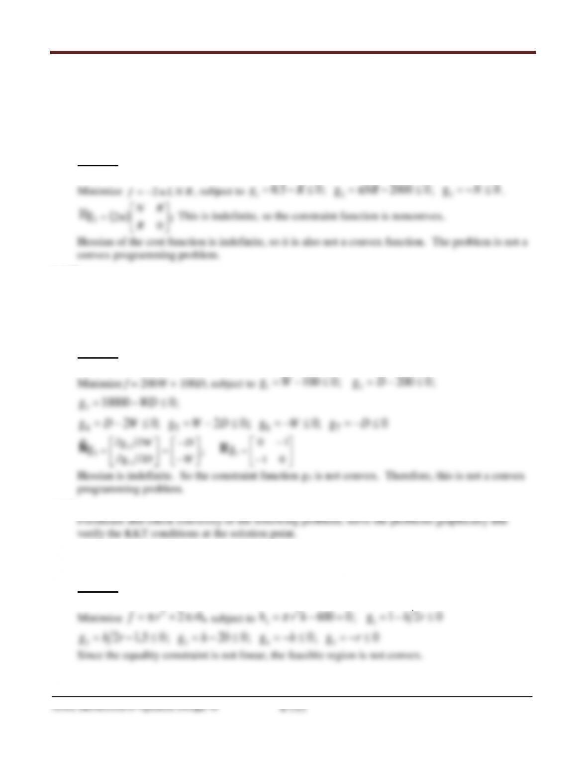
Referring to Exercise 4.85, the problem is written in the standard form as
Minimize
2
π , f RH= −
1
g2π 900 0
RH
= −≤
Chapter 4 Optimum Design Concepts
4.144_______________________________________________________________________________
Formulate and check convexity of the following problem; solve the problems graphically and
verify the KKT conditions at the solution point.
Exercise 2.4
Solution
Referring to Exercise 4.86, the problem is written in the standard form as
4.145_______________________________________________________________________________
Formulate and check convexity of the following problem; solve the problems graphically and
verify the KKT conditions at the solution point.
Exercise 2.5
Solution
Referring to Exercise 4.87, the problem is written in the standard form as
4.146_______________________________________________________________________________
Exercise 2.9
Solution
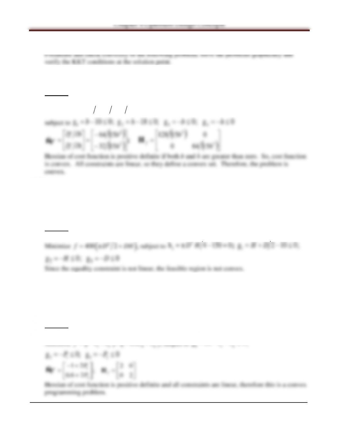
Referring to Exercise 4.91, the problem is written in the standard form as
2
2
4.147_______________________________________________________________________________
Exercise 2.10
Solution
Referring to Exercise 4.92, the problem is written in the standard form as
Minimize
( )( )
32 15 1 2 ,f hb= +
4.148_______________________________________________________________________________
Formulate and check convexity of the following problem; solve the problems graphically and
verify the KKT conditions at the solution point.
Exercise 2.12
Solution
Referring to Exercise 4.94, we have
2
2
4.149_______________________________________________________________________________
Formulate and check convexity of the following problem; solve the problems graphically and
verify the KKT conditions at the solution point.
Exercise 2.14
Solution
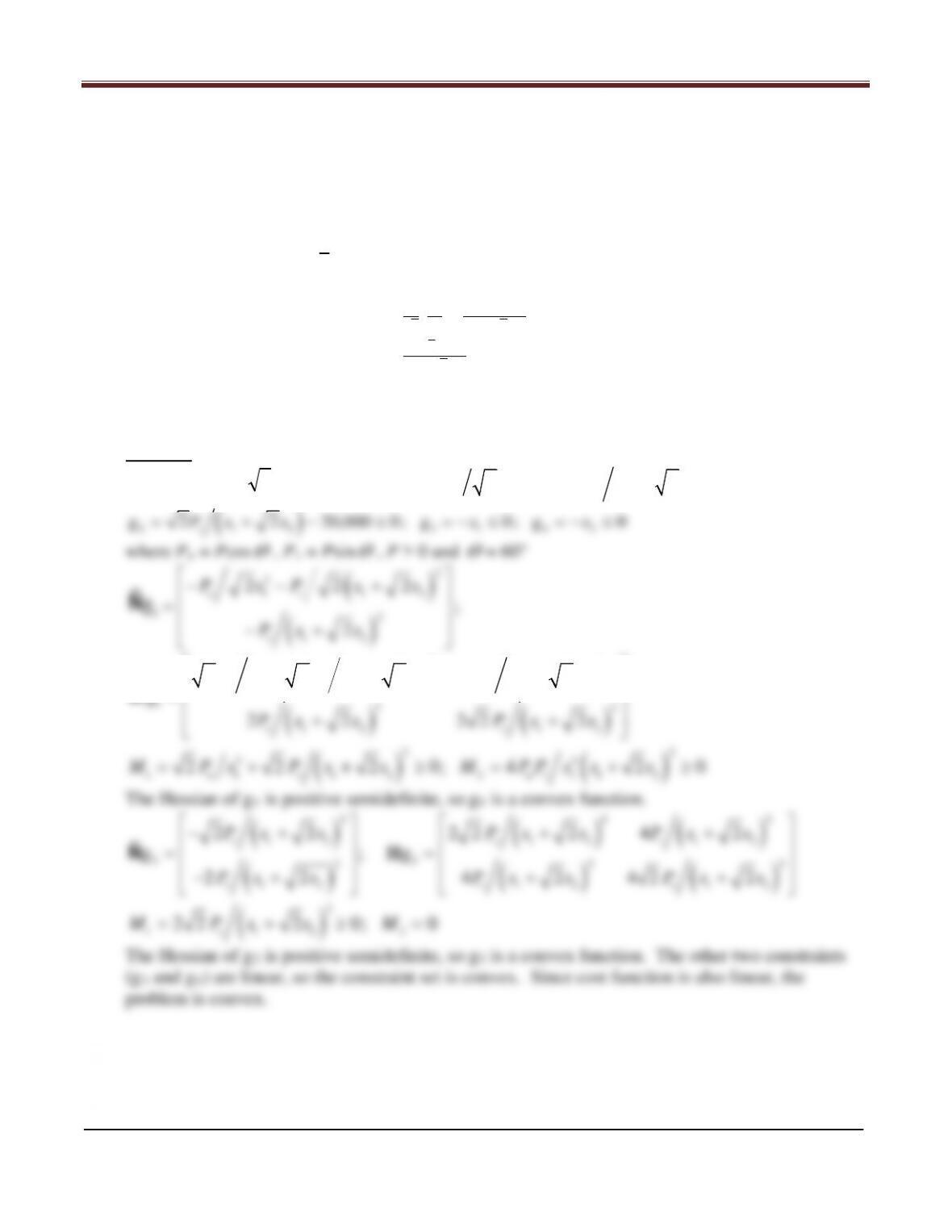
Referring to Exercise 4.96, the problem is written in the standard form as
2
2
Chapter 4 Optimum Design Concepts
Arora, Introduction to Optimum Design, 4e
4-195
Section 4.9 Engineering Design Examples
4.150_______________________________________________________________________________
The problem of minimum weight design of the symmetric three–bar truss of Fig. 2-6 is formulated
as follows:
Minimize (1,2)= 2√21+2
Subject to the constraints
g1=1
�2�
1+
�1+�22��−20,000 ≤0
g2=�2
�1+�22�−20,000 ≤0
g3=−1≤0
g4=−2≤0
Solution
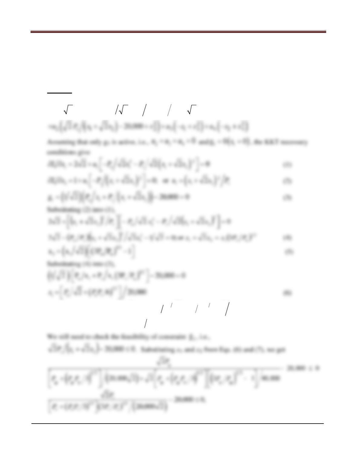
Minimize
21
22 xxf +=
, subject to
( ) ( )
1 1 12
g 1 2 2 20 000 0
uv
Px P x x ,
= ++ − ≤
/
( )
2 1 2 31 4 2
g 2 2 20,000 0; g 0; g 0
v
Px x x x= + − ≤ =−≤ =−≤
where Pu = Pcos
θ
, Pv = Psin
θ
, P > 0 and
θ
= 60°
1
gÑ
( )
( )
2
2
1 12
2
12
2 22
;
2
uv
v
P xP x x
Px x
−− +
=
−+
( ) ( )
( ) ( )
33
3
1 12 12
133
12 12
2 2 22 2
g
2 2 22 2
uv v
vv
Px Pxx Pxx
Px x Px x
++ +
=
++
H
( ) ( )
33
33
1 1 12 2 112
2 2 20; 4 20
u v uv
M Px Pxx MPPxxx= + +≥= +≥
The Hessian of g1 is positive semidefinite, so g1 is a convex function.
( )
( )
( ) ( )
( ) ( )
2 33
12 12 12
22
2 33
12 12 12
2 2 22 2 4 2
g ; g
2 2 4 2 42 2
v vv
v vv
Pxx Pxx Pxx
Px x Px x Px x
−+ + +
= =
−+ + +
HÑ
( )
3
1 12 2
2 2 2 0; 0
v
M Px x M= +≥ =
The Hessian of g2 is positive semidefinite, so g2 is a convex function. The other two constraints
(g3 and g4) are linear, so the constraint set is convex. Since cost function is also linear, the
problem is convex.
Chapter 4 Optimum Design Concepts
Arora, Introduction to Optimum Design, 4e
4-196
4.151_______________________________________________________________________________
For the three-bar truss problem of Exercise 4.150, consider the case of KKT conditions with g1 as
the only active constraint. Solve the conditions for optimum solution and determine the range for
the load angle θ for which the solution is valid.
Solution
Referring to Exercise 4.150, the Lagrange function is
( ) ( )
( )
2
121 1 2 1
2 2 1 2 2 20,000
1
L x x u Px P x x s
uv
= ++ + + − +
( )
( )
( ) ( )
22 2
2 1 2 2 313 4 24
2 2 20,000
v
u Px x suxsuxs+ + − ++−++−+
Assuming that only g1 is active, i.e.,
0
432 === uuu
and
( )
11
g0 0s= =
, the KKT necessary
conditions give
( )
22
1 1 1 12
22 2 2 2 0
uv
Lx u P x P x x
∂∂= + − − + =
(1)
( ) ( )
22
2 1 12 112
1 2 0; or 2
vv
Lx uPxx uxxP
∂∂=+ − + = = +
(2)
( ) ( )
( )
1 1 12
g 1 2 2 20,000 0
uv
Px P x x= ++ − =
(3)
Substituting (2) into (1),
( ) ( )
0222222 2
21
2
1
2
21 =
+−−
++ xxPxPPxx vuv
( )
( )
( )
21
121
2
1
2
21
32or ;0212222
uvvu
PPxxxxxxPP =+=−+−
(4)
( )
( )
12
2 1 uu
x x 2 3P P 1
= −
(5)
Substituting (4) into (3),
( )
( )
12
11
1 2 P x P x 3P P 20,000 0
u v vu
+ −=
( )
12
12 6 20,000
u uv
x P PP
= +
(6)
Substituting (6) into (5),
( ) ( )
12 12
2
3 3 1 40,000
u uv v u
x P PP P P
=+−
(7)
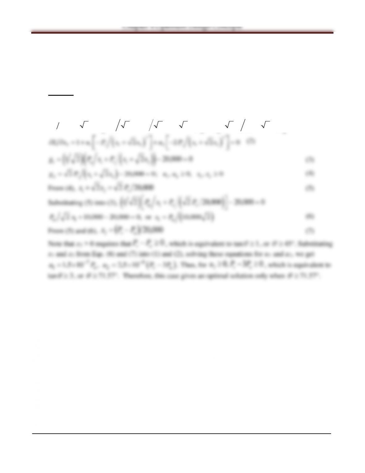
Note that
0
2
≤x
requires that
uv
PP3
, which is equivalent to
3tan 1≥
θ
, or
≥
θ
18.43°.
( ) ( )
( )
12 12
3 3 20,000 2
u uv v u
P PP P P
+
Chapter 4 Optimum Design Concepts
( )
or ,01
3
2
21 ≤−
+vvu
v
PPP
P
;3
uv
PP ≤
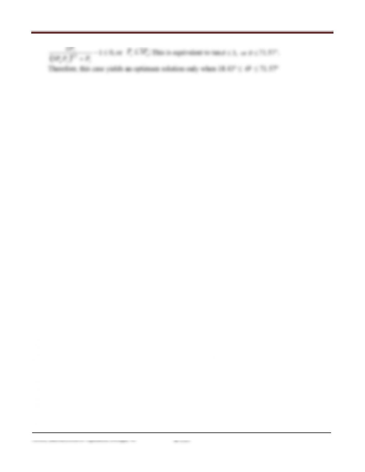
This is equivalent to tan
3, or ≤≤
θθ
71.57°.
Therefore, this case yields an optimum solution only when 18.43º ≤
θ
≤ 71.57º
Arora, Introduction to Optimum Design, 4e
4-198
4.152_______________________________________________________________________________
For the three-bar truss problem of Exercise 4.150, consider the case of KKT conditions with g1
and g2 as active constraints. Solve the conditions for optimum solution and determine the range for
the load angle θ for which the solution is valid.
Solution
Referring to Exercise 4.150, we write the KKT conditions for the case
( )
1 2 12 34
g g 0 0 and 0:ss uu== == −=
( ) ( )
22
2
1 1 1 12 2 12
22 2 2 2 2 2 0
uv v
Lx uPxP xx u Pxx
∂∂= + − − + + − + =
(1)
( ) ( )
22
2 1 12 2 12
1 2 2 20
vv
Lx u Px x u Px x
∂∂ =+ − + + − + =
(2)
( ) ( )
( )
1 1 12
g 1 2 2 20,000 0
uv
Px P x x= ++ − =
(3)
( )
2 1 2 1 2 12
g 2 2 20,000 0; , 0, , 0
v
P x x uu xx= +− = ≥ ≥
(4)
From (4),
000,2022 21 v
Pxx =+
(5)
Substituting (5) into (3),
( ) ( )
1
1 2 2 20,000 20,000 0
u vv
Px P P
+ −=
( )
11
2 10,000 20,000 0, or 10,000 2
uu
P x xP+− = =
(6)
From (5) and (6),
( )
000,20
2uv PPx −=
(7)
Note that x2 > 0 requires that
0≥−
uv
PP
, which is equivalent to tan
1≥
θ
, or
≥
θ
45°. Substituting
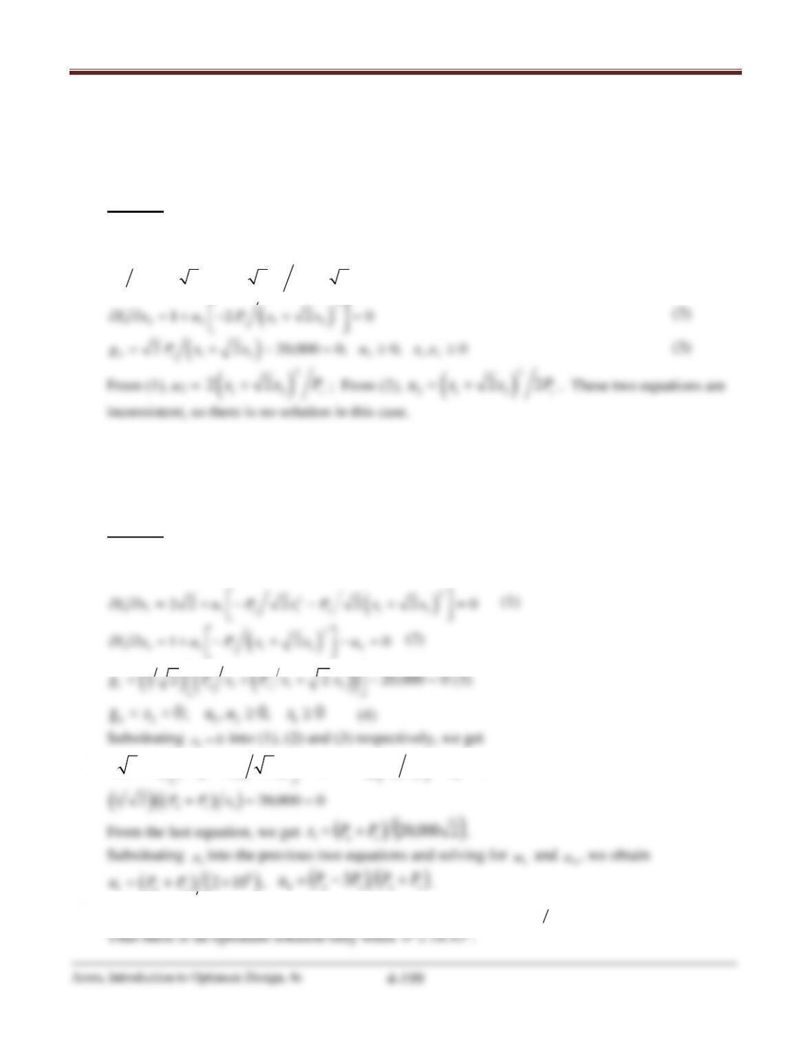
x1 and x2 from Eqs. (6) and (7) into (1) and (2), solving these equations for u1 and u2, we get
( )
79
12
1 5 10 , 2 5 10 3
u vu
u Pu P P
−−
=× =×−..
. Thus, for
03 ,0
2
≥−≥
uv
PPu
, which is equivalent to
tan
3≥
θ
, or
≥
θ
71.57°. Therefore, this case gives an optimal solution only when
≥
θ
71.57°.
Chapter 4 Optimum Design Concepts
4.153_______________________________________________________________________________
For the three-bar truss problem of Exercise 4.150, consider the case of KKT conditions with g2 as
the only active constraint. Solve the conditions for optimum solution and determine the range for
the load angle θ for which the solution is valid.
Solution
Ref. to Exercise 4.150, the KKT conditions for the case
( )
2 2 1 34
g 0 0 and 0s u uu= = = = =
,
are
( )
2
1 2 12
22 2 2 0
v
Lx u P x x
∂∂= + − + =
(1)
( )
2
2 2 12
12 2 0
v
Lx u P x x
∂∂ =+ − + =
(2)
( )
2 1 2 2 12
g 2 2 20,000 0, 0, , 0
v
P x x u xx= +− =≥ ≥
(3)
From (1), u2 =
( )
2
12
22
v
x xP+
; From (2),
( )
2
21 2
22
v
ux x P= +
. These two equations are
inconsistent, so there is no solution in this case.
4.154_______________________________________________________________________________
For the three-bar truss problem of Exercise 4.150, consider the case of KKT conditions with g1
and g4 as active constraints. Solve the conditions for optimum solution and determine the range for
the load angle θ for which the solution is valid.
Solution
Referring to Exercise 4.150, we write the KKT conditions for this case,
( )
1 4 14 2 3
g g 0 0 and 0,ss uu= = = = = =
as
( )
2
2
1 1 1 12
22 2 2 2 0
uv
Lx u P x P x x
∂∂= + − − + =
(1)
( )
2
2 1 124
1 20
v
Lx u P x x u
∂∂ =+ − + − =
(2)
( ) ( )
( )
1 1 12
g 1 2 2 20,000 0
uv
Px Px x
= ++ − =
(3)
4 2 12 1
g 0; , 0, 0x uu x== ≥≥
(4)
0
=x
2
( )
( )
22
1 1 1 14
2 2 2 0; 1 0
uv v
u P P x uPx u
+ −− = − − =
( )
( )
( )
1
1 2 20,000 0
uv
PPx+−=
From the last equation, we get
( )
( )
2000,20
1vu PPx +=
.
Substituting
1
x
into the previous two equations and solving for
1
u
and
4
u
, we obtain
( )
( )
8
1
2 10 ,
uv
u PP=+×
( ) ( )
vuvu
PPPPu +−= 3
4
.
Now
0
4
≥u
requires that
03 ≥− vu PP
which is equivalent to tan
13≤
θ
, or
≤
θ
18.43°.