
CHAPTER
4
Optimum Design Concepts
Optimality Conditions
Section 4.2 Review of Some Basic Calculus Concepts
4.1_________________________________________________________________________________
Answer True or False.
2. A function cannot have more than one global minimum point. False
4. A function defined on an open set cannot have a global minimum. False
6. Gradient of a function at a point gives a local direction of maximum decrease in the function. False
8. The Hessian matrix for a function is calculated using only the first derivatives of the function. False
10. Taylor series expansion can be written at a point where the function is discontinuous. False
12. Linear Taylor series expansion of a complicated function at a point is only a good local
approximation for the function. True
14. For a given x, the quadratic form defines a vector. False
16. A symmetric matrix is positive definite if its eigenvalues are nonnegative. False
18. All eigenvalues of a negative definite matrix are strictly negative. True
20. A positive definite quadratic form must have positive value for any x ≠ 0. True

Arora, Introduction to Optimum Design, 4e
4-2
4.2_________________________________________________________________________________
Write the Taylor series expansion for the following function up to quadratic terms.
cosx about the point x* =
4
π
Solution
( ) ( ) ( ) ( ) ( )
( ) ( ) ( )
( ) ( )( ) ( )( )
( ) ( )
( )
( )
( )
2
22
cos ; 4 cos 4 1 2 ; ‘ 4 sin 4 1 2 ;
“ 4 cos 4 1 2 ; ‘ 0.5 “ cos
1 2 1 2 4 0.5 1 2 4 1.0444 0.15175 0.35355
fx xf f
f fx fx fx xx f x xx x
x x xx
∗ ∗∗ ∗∗
= = = =−=−
=− =− = + −+ −
= − − +− − = − −
ππ π π
ππ
ππ
4.3_________________________________________________________________________________
Write the Taylor series expansion for the following function up to quadratic terms.
cosx about the point x* =
3
π
Solution
( ) ( ) ( ) ( ) ( )
( ) ( ) ( )
( ) ( )( ) ( )( )
( ) ( )
( ) ( )( )
2
22
cos ; 3 cos 3 1 2; ‘ 3 sin 3 3 2;
“ 3 cos 3 1 2; ‘ 0.5 “
cos 1 2 3 2 3 0.5 1 2 3 1.1327 0.34243 0.25
fx xf f
f fx fx fx xx f x xx
x x x xx
∗ ∗∗ ∗∗
= = = =−=−
=− =− = + −+ −
= − − +− − = − −
ππ π π
ππ
ππ
4.4 _________________________________________________________________________________
Write the Taylor series expansion for the following function up to quadratic terms.
sinx about the point x* =
6
π
Solution
( ) ( ) ( ) ( ) ( )
( ) ( ) ( )
( ) ( )( ) ( )( )
( )
( ) ( )( )
2
22
sin ; 6 sin 6 1 2; ‘ 6 cos 6 3 2;
“ 3 cos 3 1 2; ‘ 0.5 “
sin 1 2 3 2 6 0.5 1 2 6 0.02199 1.12783 0.25
fx xf f
f fx fx fx xx f x xx
x x x xx
∗ ∗∗ ∗∗
= = = = = −
=− =− = + −+ −
=− − +− − =− + −
ππ ππ
ππ
ππ
Chapter 4 Optimum Design Concepts: Optimality Conditions
4.5_________________________________________________________________________________
Write the Taylor series expansion for the following function up to quadratic terms.
sin x about the point x∗=π4
�
Solution
( ) ( ) ( ) ( ) ( )
( ) ( ) ( )
( ) ( )( ) ( )( )
( )
( )
( )
( )
( )
( )
( )
2
222
22 2
sin ; 4 sin 4 1 2 ; ‘ 4 cos 4 1 2 ;
“ 4 sin 4 1 2 ; ‘ 0.5 “ sin
1 2 1 2 4 0.5 1 2 4 1 4 2 4 32 2
1 4 32 1 4 2 2 0.06634 1.2625 0.35355
fx x f f
f fx fx fx xx f x xx x
x x x xx
xx x x
∗ ∗∗ ∗∗
= = = = = −
=− =− = + −+ −
= + − + − − = +− − + −
= − − ++ − = + −
ππ π π
ππ
π π π ππ
ππ π
4.6 _________________________________________________________________________________
Write the Taylor series expansion for the following function up to quadratic terms.
about the point x*=0
Solution
( ) ( ) ( ) ( ) ( ) ( ) ( )
( )
( ) ( ) ( )
( )
( )
( ) ( )
2
2
00 0 2
; ‘ “ ; 0 ‘ 0 “ 0 1
‘ 0.5 “
0 0.5 0 1 0.5
xx
x
fx e fx f x f x e f f f
fx fx fx xx f xxx
e e ex ex x x
∗ ∗∗ ∗
= = = = = = =
= =+ =−+ −
= + − + − =++
4.7 _________________________________________________________________________________
Write the Taylor series expansion for the following function up to quadratic terms.
about the point x*=2
Solution
( ) ( ) ( )
( ) ( ) ( )
2
, 2; ‘ ; “ ; ‘ “ 7 389
x xx
fxex fxefxefx fx fx e .
∗ ∗∗ ∗
= = = = = = = =
( )
( ) ( ) ( ) ( ) ( )
2
‘ 05 “
fx fx fx xx .f x xx
∗ ∗∗ ∗∗
= + −+ −
Arora, Introduction to Optimum Design, 4e
4-4
4.8_________________________________________________________________________________
Write the Taylor series expansion for the following function up to quadratic terms.
(1,2)=101
4−201
22+102
2+1
2−21+ 5 about the point (1,1). Compare approximate
and exact values of the function at the point (1.2,0.8).
Solution
( ) ( )
( ) ( )
( )
( ) ( )( ) ( ) ( )( )
( ) ( ) ( )
4 2 22
1 2 1 12 2 1 1
32
1 12 1 1 2 1
12 12
2
12 1
12
, 10 20 10 2 5; 1, 1
40 40 2 2 120 40 2 40
, ; ,
20 20 40 20
, 0 5
0 82
4; ;
0
T
T
f x x x xx x x x x
x xx x x x x
fxx xx
xx x
fxx fx f x xx xx x xx
fx fx x
∗
∗ ∗∗ ∗∗∗
∗∗ ∗
= − + +− + =
− +− − +−
= =
−+ −
= + −+ − −
−
= = =
H
.H
H
Ñ
Ñ
Ñ
( ) ( )
( ) ( )
( )
( ) ( )
11
22
1
1 2 1 1 12 2 2
2
22
40
40 20
11
82 40
, 4 41 42 40 20 10 15
11
40 20
1 2, 0.8 8 136; 1 2, 0.8 7 64; Error 0 496
T
xx
f x x x x xx x x
xx
f f ff
−
−−
−
=+ = −− +++
−−
−
= = =−=.. .. .
Determine the nature of the following quadratic forms.
4.9_________________________________________________________________________________
Determine the nature of the following quadratic form.
()=1
2+ 412+ 213−72
2−623+ 53
2
Solution
( )
[ ]
2 22
1 12 13 2 23 3
1
123 2
3
4 2 76 5
12 1 12 1
273 ; 273
1 35 1 35
F x xx xx x x x x
x
xx x x
x
=+ + −− +
= −− = −−
−−
x
A
Chapter 4 Optimum Design Concepts: Optimality Conditions
4.10________________________________________________________________________________
Determine the nature of the following quadratic form.
()= 21
2+ 22
2−512
Solution
( )
[ ]
1
22
1 2 12 1 2
2
2 25
225 25 2
x
F x x xx x x x
−
=+− =
−
.
x.
4.13_____________________________________________________________________________
Determine the nature of the following quadratic form.
()=1
2− 2
2+ 412
Solution
( )
[ ]
1
22
1 2 12 1 2
2
12
12
421
12
; Principal Minors: 1 0; 5 0
21
x
F x x xx x x x
MM
=−+ =
−
= => =−<
−
x
A
Since M1 > 0 and M2 < 0, the matrix is indefinite and so is the quadratic form.
4.14 ________________________________________________________________________________
Determine the nature of the following quadratic form.
()=1
2− 2
2+3
2−223
Solution
( )
[ ]
222
1 2 3 23
1
123 2
3
2
10 0 10 0
011 ; 011
0 11 0 11
F x x x xx
x
xxx x
x
=−+−
= −− = −−
−−
x
A
Principal Minors: M1 = 1 > 0, M2 = -1 < 0, M3 =
( )
2111 −=−−=A
< 0
Since M1 > 0, M2 < 0 and M3 < 0, so the quadratic form is indefinite.
4.15________________________________________________________________________________
Determine the nature of the following quadratic form.
()=1
2−212+ 22
2
Solution
( )
[ ]
1
22
1 12 2 1 2
2
11
22 12
x
F x xx x x x x
−
=− +=
−
x
11
−
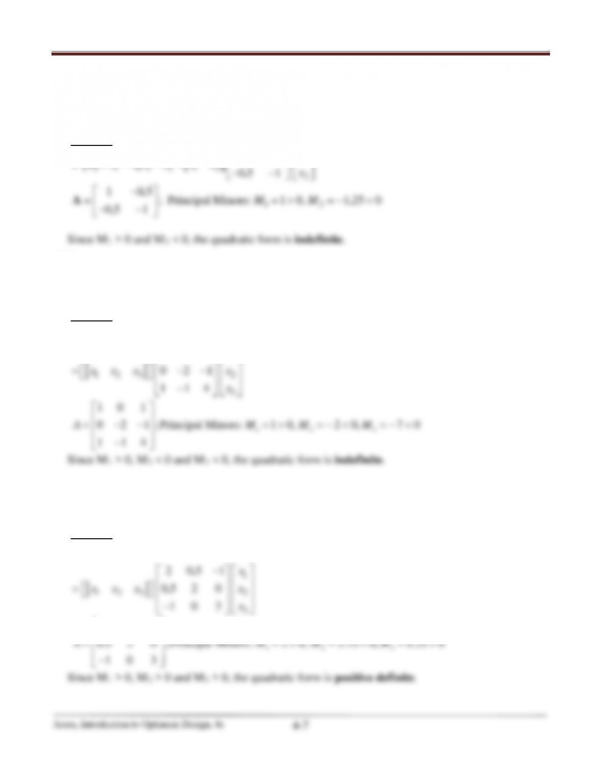
Chapter 4 Optimum Design Concepts: Optimality Conditions
4.16_____________________________________________________________________________
Determine the nature of the following quadratic form.
()=1
2− 12− 2
2
Solution
( )
[ ]
1
22
1 12 2 1 2
2
1 05
05 1
x
F x xx x x x x
−
=− −=
−−
.
x.
1 05 ; Principal Minors: 1 0, 1 25 0
−
.
4.17_____________________________________________________________________________
Determine the nature of the following quadratic form.
()=1
2+ 213−22
2+ 43
2−223
Solution
( )
2 22
1 13 2 3 23
1
2 242
10 1
F xxxxxxx
x
=+ −+−
x
12 3
10 1
0 2 1 ; Principal Minors: 1 0, 2 0, 7 0
1 14
A MM M
= − − => =−< =−<
−
Since M1 > 0, M2 < 0 and M3 < 0, the quadratic form is indefinite.
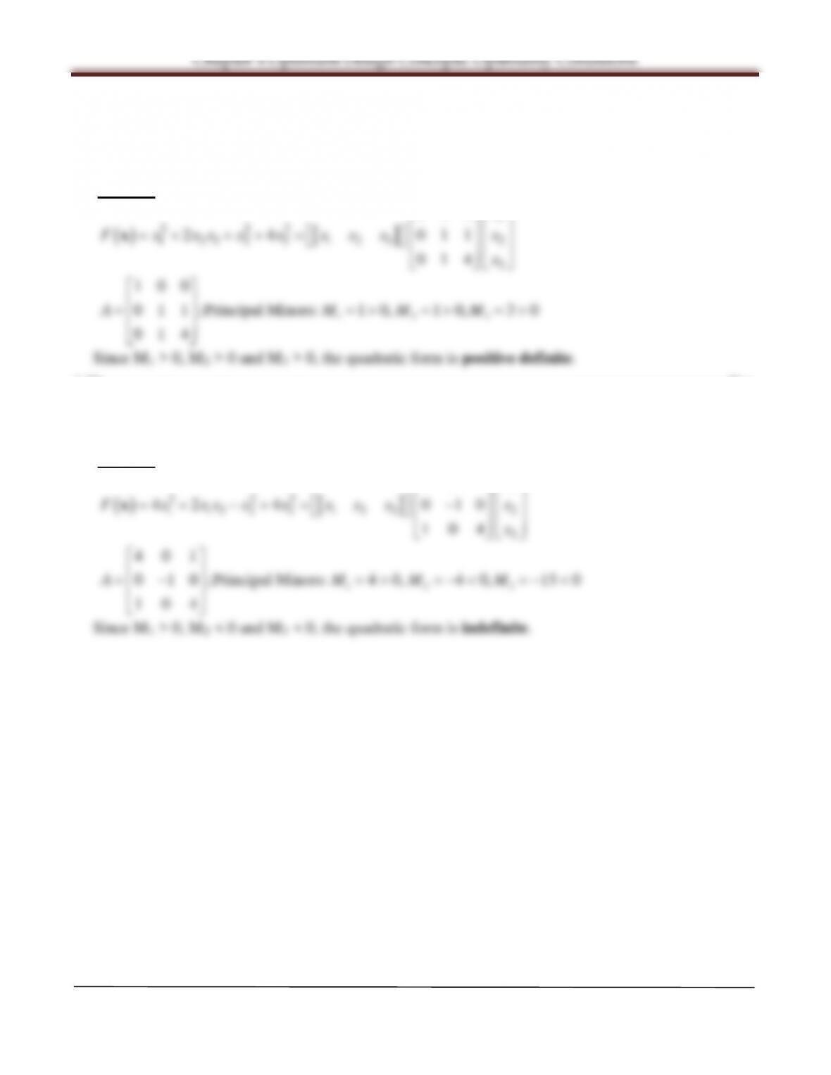
4.18_____________________________________________________________________________
Determine the nature of the following quadratic form.
()= 21
2+12+ 22
2+ 43
2−213
Solution
( )
[ ]
2 22
1 12 2 3 13
1
123 2
3
2 242
2 05 1
05 2 0
10 3
F x xx x x xx
x
xx x x
x
=+ ++−
−
=
−
x
.
.
12 3
2 0.5 1
0.5 2 0 ; Principal Minors: 2 0, 3.75 0, 9.25 0
10 3
A MM M
−
= => =>=>
−
Since M1 > 0, M2 > 0 and M3 > 0, the quadratic form is positive definite.
Arora, Introduction to Optimum Design, 4e
4-8
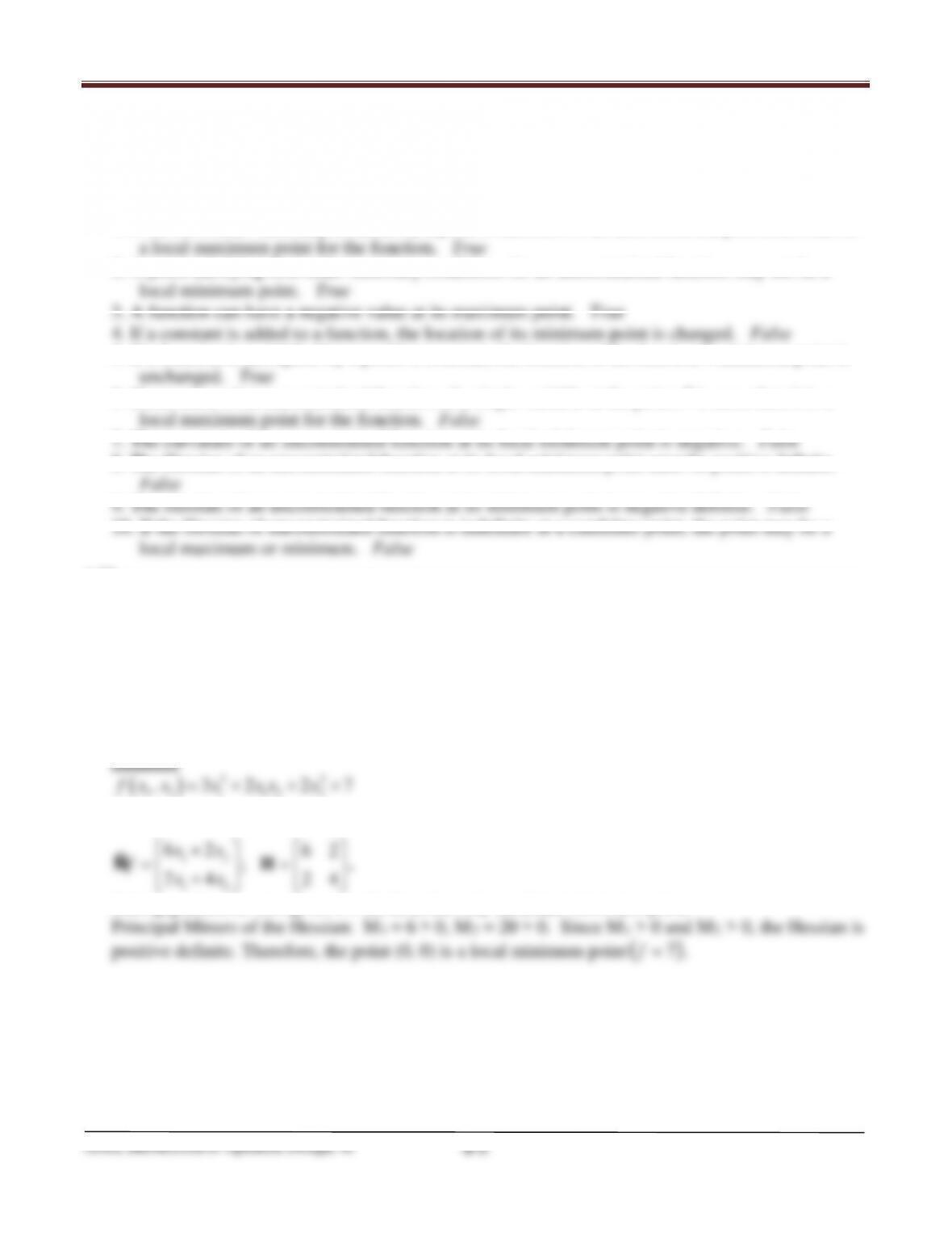
4.19_____________________________________________________________________________
Determine the nature of the following quadratic form.
()=1
2+ 223+2
2+ 43
2
Solution
( )
[ ]
1
2 22
1 23 2 3 1 2 3 2
3
100
2 4 011
014
x
F xxxxx xxx x
x
=+ ++ =
x
1 23
100
0 1 1 ;Principal Minors: 1 0, 1 0, 3 0
014
A MMM
= => =>=>
Since M1 > 0, M2 > 0 and M3 > 0, the quadratic form is positive definite.
4.20_____________________________________________________________________________Det
Determine the nature of the following quadratic form.
()= 41
2+ 213− 2
2+ 43
2
Solution
( )
[ ]
1
2 22
1 13 2 3 1 2 3 2
3
401
4 2 4 0 10
104
x
F xxxxx xxx x
x
= + −+ = −
x
12 3
401
0 1 0 ;Principal Minors: 4 0, 4 0, 15 0
104
A MM M
= − = > =−< =− <
Since M1 > 0, M2 < 0 and M3 < 0, the quadratic form is indefinite.
Chapter 4 Optimum Design Concepts: Optimality Conditions
Section 4.4 Optimality Conditions: Unconstrained Problems
4.21________________________________________________________________________________
Answer True or False.
1. If the first–order necessary condition at a point is satisfied for an unconstrained problem, it can be
2. A point satisfying first-order necessary conditions for an unconstrained function may not be a
5. If a function is multiplied by a positive constant, the location of the function’s minimum point is
6. If curvature of an unconstrained function of a single variable at the point x* is zero, then it is a
8. The Hessian of an unconstrained function at its local minimum point must be positive definite.
4.22________________________________________________________________________________
Find stationary points for the following function (use a numerical method such as the Newton-
Raphson method, or a software package like Excel, MATLAB, and Mathematica, if needed). Also
determine the local minimum, local maximum, and inflection points for the function (infection
points are those stationary points that are neither minimum nor maximum).
( )
22
1 2 1 12 2
, 3 2 2 7f x x x xx x=+ ++
Solution
( )
( )
22
1 2 1 12 2
12
12
, 3 2 2 7
The gradient and Hessian of are
62 62
;
24 24
f x x x xx x
f
xx
fxx
=+ ++
+
= =
+
x
H.Ñ
Setting gradient to zero gives x = (0, 0) as the only candidate minimum point.
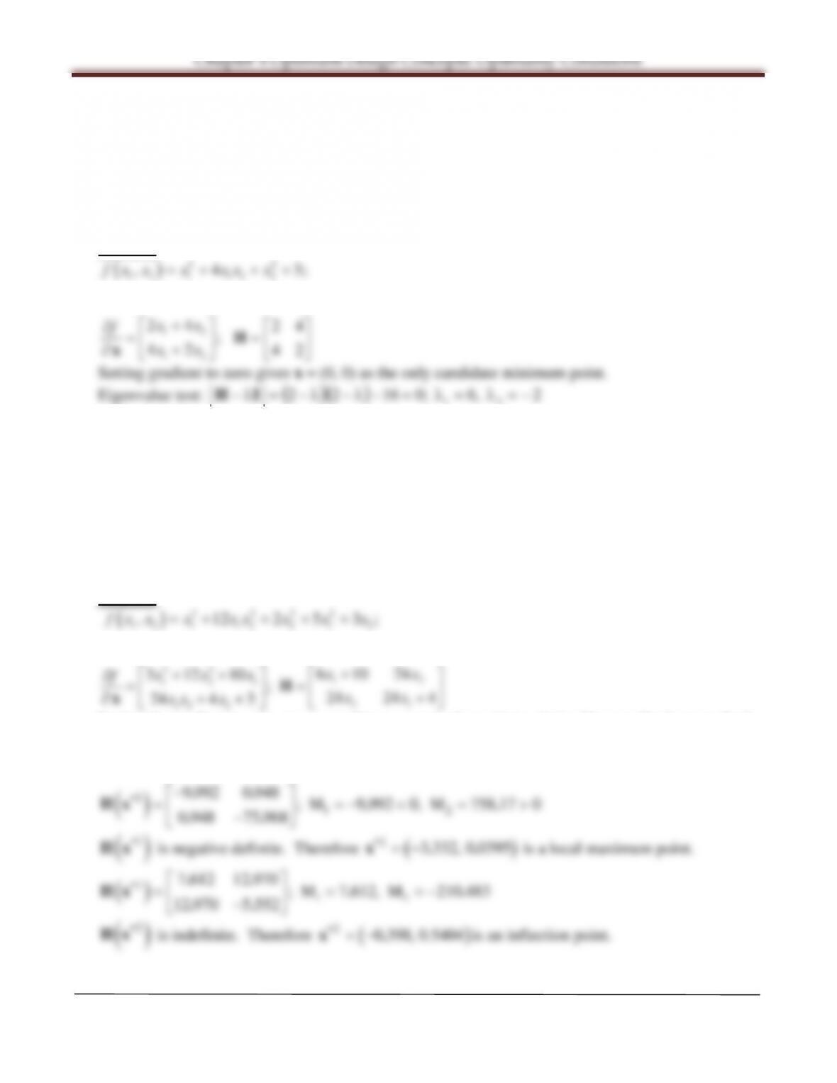
Arora, Introduction to Optimum Design, 4e
4-10
4.23________________________________________________________________________________
Find stationary points for the following function (use a numerical method such as the Newton-
Raphson method, or a software package like Excel, MATLAB, and Mathematica, if needed). Also
determine the local minimum, local maximum, and inflection points for the function (infection
points are those stationary points that are neither minimum nor maximum).
(1,2)=1
2+ 412+2
2+ 3
Solution
( )
( )
22
1 2 1 12 2
12
12
, 4 3;
The gradient and Hessian of are
24 24
;
42 42
f x x x xx x
f
xx
f
xx
=+ ++
+
∂= =
+
∂
x
H
x
21
Therefore, the Hessian is indefinite and second order necessary condition is violated. The stationary
point (0, 0) is an inflection point.
4.24________________________________________________________________________________
Find stationary points for the following function (use a numerical method such as the Newton-
Raphson method, or a software package like Excel, MATLAB, and Mathematica, if needed). Also
determine the local minimum, local maximum, and inflection points for the function (infection
points are those stationary points that are neither minimum nor maximum).
(1,2)=1
3+1212
2+ 22
2+ 51
2+ 32
Solution
( )
( )
3 222
1 2 1 12 2 1 2
, 12 2 5 3 ;
The gradient and Hessian of are
f x x x xx x x x
f
=+ +++
x
22
12
1 21
21
12 2
6 10 24
3 12 10 ; 24 24 4
24 4 3
xx
xxx
f
xx
xx x
+
++
∂= =
+
∂++
x
Setting the gradient to zero gives a nonlinear system of equations. Using Newton-Raphson method
or any nonlinear equation solver, we find two solutions, as
( ) ( )
12
3 332, 0.0395 ; 0 398, 0.5404
∗∗
=−=−x. x.
1
9 992 0 948 ; M 9 992 0, M 758 17 0
∗−
..
Chapter 4 Optimum Design Concepts: Optimality Conditions
4.25________________________________________________________________________________
Find stationary points for the following function (use a numerical method such as the Newton-
Raphson method, or a software package like Excel, MATLAB, and Mathematica, if needed). Also
determine the local minimum, local maximum, and inflection points for the function (infection
points are those stationary points that are neither minimum nor maximum).
(1,2)= 51− 1
2216
⁄+2
241
⁄
Solution
( )
( )
22
1 2 1 12 2 1
22 23 2
12 2 1 2 2 1 1 2 1
22
1 21 1 21 1
, 5 16 4
The gradient and Hessian of are
5 84 82 82
;
16 2 8 2 1 2
f x x x xx x x
f
xx x x x x x x x x
fx xx x x x x
=−+
− − −+ − −
∇= =
− + −−
x
H
When
fÑ
is set to zero the second equation gives
3
21
8xx=
.
Substituting into the first equation, we get
44 4
For the first point
( )
8 ,4
( ) ( )
( ) ( )
085M ,021M
;
8143
4321
421162884
1628846426488
21 <−=<−=
−−
−−
=
−−
−−+−
=H
Since H is indefinite, the second order necessary condition is violated. Thus, point
( )
8 ,4
is an
inflection point.
For the second point
( )
8 ,4 −−
,
( ) ( ) ( ) ( ) ( )
( ) ( ) ( ) ( )
085M ,021M
;
8143
4321
421162884
1628846426488
21 <−=>=
−
=
−−−−−
−−−−−+−−
=H
.
Since H is indefinite, the second order necessary condition is violated. Thus, point
( )
8 ,4 −−
is an
inflection point.
Arora, Introduction to Optimum Design, 4e
4-12
4.26________________________________________________________________________________
Find stationary points for the following function (use a numerical method such as the Newton-
Raphson method, or a software package like Excel, MATLAB, and Mathematica, if needed). Also
determine the local minimum, local maximum, and inflection points for the function (infection
points are those stationary points that are neither minimum nor maximum).
()=cos
Solution
( )
( )
cos
The necessary condition gives ‘ sin 0
fx x
fx x
=
=−=
The solution of necessary condition gives:
, 0, 1, 2,xnn=π= ±±
…
( ) ( )
…, 2, 1, 0, ,12For cos“±±=π+=−= nnxxxf ;
( ) ( )
[ ]
0112n cos“.>=π+−=xf
( )
…, 2, 1, 0, ,12 Thus, ±±=π+= nnx
are local minimum points
( )
1−=f
.
For
( ) ( )
2 , 0, 1, 2, … “ cos 2 1 0x nn fx n= π = ± ± =− π=−<.
Thus,
2 , 0, 1, 2, … x nn=π= ±± .
are local maximum points
( )
1=f
.
4.27________________________________________________________________________________
Find stationary points for the following function (use a numerical method such as the Newton-
Raphson method, or a software package like Excel, MATLAB, and Mathematica, if needed). Also
determine the local minimum, local maximum, and inflection points for the function (infection
points are those stationary points that are neither minimum nor maximum).
(1,2)=1
2+12+2
2
Solution
( )
2
221
2
121 , xxxxxxf ++=
The gradient and Hessian of
( )
xf
are
12
221
xx
+
Chapter 4 Optimum Design Concepts: Optimality Conditions
4.28________________________________________________________________________________
Find stationary points for the following function (use a numerical method such as the Newton-
Raphson method, or a software package like Excel, MATLAB, and Mathematica, if needed). Also
determine the local minimum, local maximum, and inflection points for the function (infection
points are those stationary points that are neither minimum nor maximum).
()=2−
Solution
( )
x
exxf
−
=
2
Therefore, x = 0, 2 are the stationary points.
( )
( )
( )
( )
22
“ 2 2 2 42
“ 0 2 0. Therefore, 0 is a local minimum point. f* = 0.
“ 2 0 27067 0. Therefore, 2 is a local maximum point. f* = 0.541.
xxxx x
f x e xe xe x e x x e
fx
fx
−−−− −
=−−+=−+
=>=
=−< =.
4.29________________________________________________________________________________
Find stationary points for the following function (use a numerical method such as the Newton-
Raphson method, or a software package like Excel, MATLAB, and Mathematica, if needed). Also
determine the local minimum, local maximum, and inflection points for the function (infection
points are those stationary points that are neither minimum nor maximum).
(1,2)=1+10 (12)⁄+ 52
Solution
( ) ( )
221121 510 , xxxxxxf ++=
The necessary condition gives:
( ) ( )
105 ,10or ;0510 ;0101
2
2
2
2
===+−=∂∂=−=∂∂ xxxxxxxfxxxf
Arora, Introduction to Optimum Design, 4e
4-14
4.30________________________________________________________________________________
Find stationary points for the following function (use a numerical method such as the Newton-
Raphson method, or a software package like Excel, MATLAB, and Mathematica, if needed). Also
determine the local minimum, local maximum, and inflection points for the function (infection
points are those stationary points that are neither minimum nor maximum).
(1,2)=1
2−21+ 42
2−82+ 6
Solution
( )
22
12 1 1 2 2
, 2486fxx x x x x=−+ −+
The gradient and Hessian are given as
1
2
22 20
;
88 08
x
fx
−
= =
−
HÑ
.
Solution of
fÑ
= 0 gives
( )
1 ,1=
∗
x
. For the Hessian H, M1 = 2 > 0, M2 = 16 > 0; so it is positive
definite, and
( )
1 1,
is a local minimum point
( )
1=f
.
4.31________________________________________________________________________________
Find stationary points for the following function (use a numerical method such as the Newton-
Raphson method, or a software package like Excel, MATLAB, and Mathematica, if needed). Also
determine the local minimum, local maximum, and inflection points for the function (infection
points are those stationary points that are neither minimum nor maximum).
(1,2)= 31
2−212+ 52
2+ 82
Solution
( )
2
2
221
2
121 8523 xxxxxx,xf ++−=
The gradient and Hessian are given as
12
12
62 62
;
2 10 8 2 10
xx
fxx
−−
= =
−+ + −
HÑ
.
Solution of
0f=Ñ
gives
( )
2 7, 6 7
∗=−−x
. For the Hessian, M1 = 6 > 0, M2 = 56 > 0, so it is
positive definite, and the point
( )
7672 −− ,
is a local minimum point
24
()
7
f= −
.
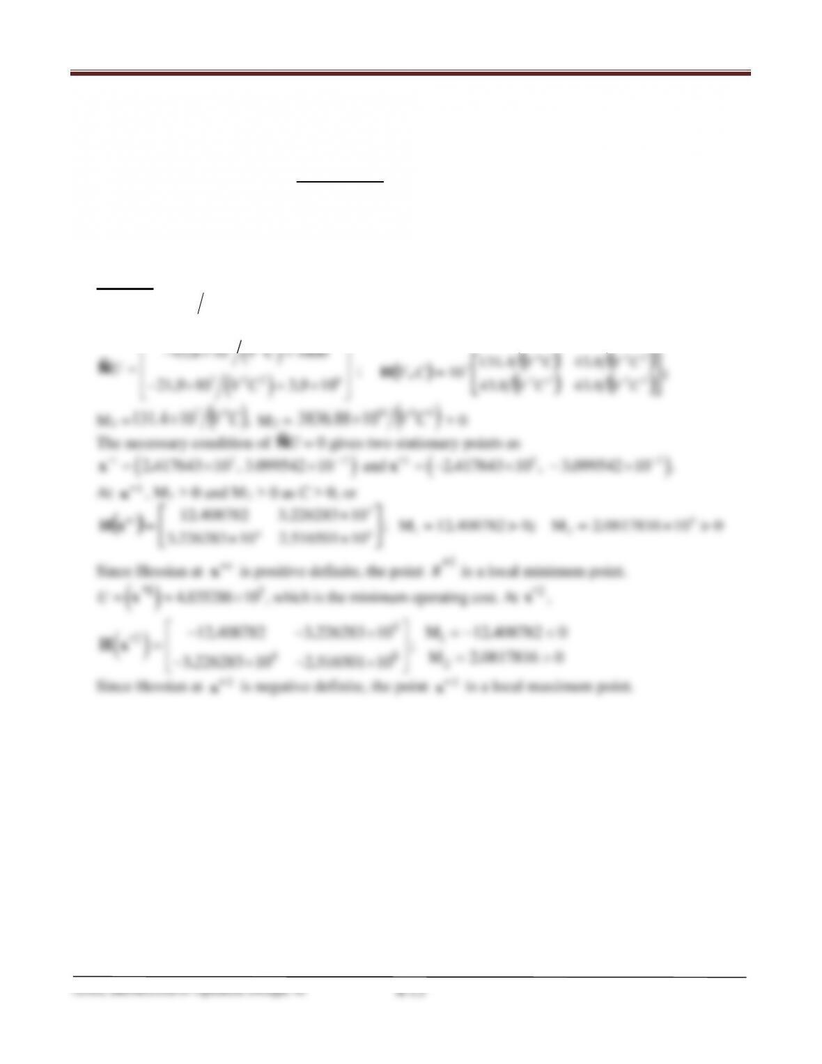
Chapter 4 Optimum Design Concepts: Optimality Conditions
4.32________________________________________________________________________________
The annual operating cost U for an electrical line system is given by the following expression
=(21.9 × 10⁷)
2+(3.9 × 10⁶)+1000
where V = line voltage in kilovolts and C = line conductance in mhos. Find stationary points for the
function, and determine V and C to minimize the operating cost.
Solution
( ) ( ) ( )
VCCVU 1000109310921
627
+×+×= ..
The gradient and Hessian are given as
( )
( )
73
7 22 6
43 8 10 1000
21 9 10 3 9 10
VC
U
VC
−× +
=
− × +×
.
..
Ñ
;
( )
( ) ( )
( ) ( )
; ,H
=2323
234
7
843843
8434131
10 CVCV
CVCV
CV ..
..
M1 =
( )
,104131
47
CV. ×
M2 =
( )
4614
10883836 CV. ×
> 0
The necessary condition of
UÑ
= 0 gives two stationary points as
( ) ( )
1 2 22 2 2
2 417643 10 , 3.099542 10 and 2 417643 10 , 3 099542 10 .
∗ −∗ −
= × × =− ×− ×x. x . .
At
1∗
x
, M1 > 0 and M2 > 0 as C > 0, or
( )
01008178162M040878212M ;
105165012102262833
10226283340878212 9
21
84
4
1>×=>=
××
×
=
∗.;.
..
..
xH
Since Hessian at
1∗
x
is positive definite, the point
1∗
x
is a local minimum point.
( )
52
4 835286 10 , which is the minimum operating cost. At , U
∗
= = ×
*1
x. x
( )
4
1
2
48
2
M 12 408782 0
12 408782 3 226283 10 ; M 2 0817816 0
3 226283 10 2 516501 10
∗
=−<
− −×
=
= >
− ×− ×
.
..
Hx .
..
Since Hessian at
2∗
x
is negative definite, the point
2∗
x
is a local maximum point.
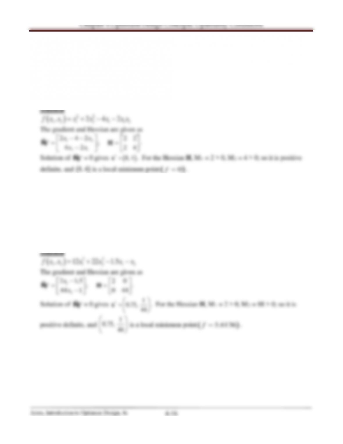
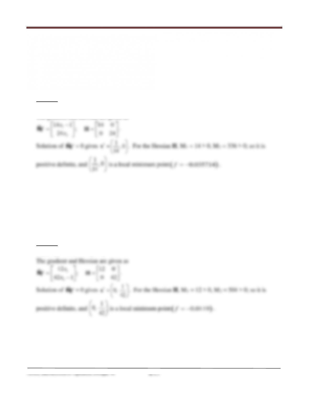
Chapter 4 Optimum Design Concepts: Optimality Conditions
4.35 ________________________________________________________________________________
Find stationary points for the following function (use a numerical method such as the Newton-
Raphson method, or a software package like Excel, MATLAB, and Mathematica, if needed). Also
determine the local minimum, local maximum, and inflection points for the function (infection
points are those stationary points that are neither minimum nor maximum).
(1,2)= 71
2+122
2− 1
Solution
( )
22
12 1 2 1
, 7 12fxx x x x=+−
The gradient and Hessian are given as
1
2
14 1 14 0
;
24 0 24
x
fx
−
= =
HÑ
.
Solution of
fÑ
= 0 gives
1, 0
14
∗
=
x
. For the Hessian H, M1 = 14 > 0, M2 = 336 > 0; so it is
positive definite, and
1, 0
14
is a local minimum point
( )
0.035714f= −
.
4.36 _______________________________________________________________________________
Find stationary points for the following function (use a numerical method such as the Newton-
Raphson method, or a software package like Excel, MATLAB, and Mathematica, if needed). Also
determine the local minimum, local maximum, and inflection points for the function (infection
points are those stationary points that are neither minimum nor maximum).
(1,2)=121
2+212
2− 2
Solution
( )
22
12 1 2 2
, 12 21fxx x x x=+−
fÑ
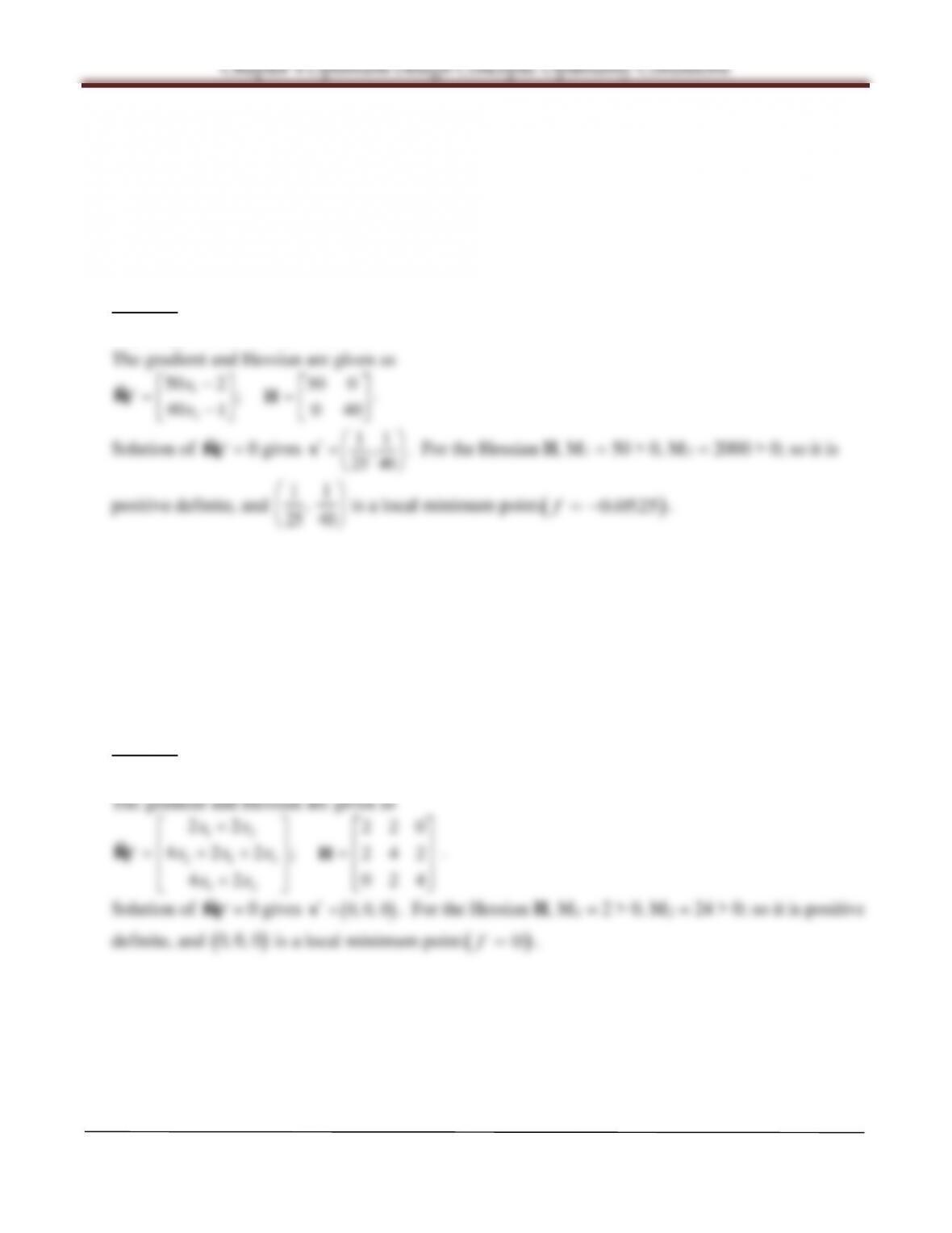
Arora, Introduction to Optimum Design, 4e
4-18
4.37 ________________________________________________________________________________
Find stationary points for the following function (use a numerical method such as the Newton-
Raphson method, or a software package like Excel, MATLAB, and Mathematica, if needed). Also
determine the local minimum, local maximum, and inflection points for the function (infection
points are those stationary points that are neither minimum nor maximum).
(1,2)=251
2+202
2−21− 2
Solution
( )
22
12 1 2 1 2
, 25 20 2fxx x x x x= + −−
4.38 ________________________________________________________________________________
Find stationary points for the following function (use a numerical method such as the Newton-
Raphson method, or a software package like Excel, MATLAB, and Mathematica, if needed). Also
determine the local minimum, local maximum, and inflection points for the function (infection
points are those stationary points that are neither minimum nor maximum).
(1,2,3)=1
2+ 22
2+ 23
2+ 212+ 223
Solution
( )
222
1 2 3 1 2 3 12 23
,, 222 2fxxxxxxxxxx=+++ +
Chapter 4 Optimum Design Concepts: Optimality Conditions
4.39 ________________________________________________________________________________
Find stationary points for the following function (use a numerical method such as the Newton-
Raphson method, or a software package like Excel, MATLAB, and Mathematica, if needed). Also
determine the local minimum, local maximum, and inflection points for the function (infection
points are those stationary points that are neither minimum nor maximum).
(1,2)= 81
2+ 82
2−80�1
2+2
2−202+100 −80�1
2+2
2+202+100 −51−52
Solution
( )
2 2 22 22
12 1 2 12 2 12 2 1 2
, 8 8 80 20 100 80 20 100 5 5fxx x x xx x xx x x x= + − +− + − ++ + − −
;
The gradient is given as
( ) ( )
( ) ( )
11
22 22
22
1 11 2 2 11 2 2
11
22 22
22
2 2 12 2 2 12 2
16 80 20 10 80 20 10 5
;
16 40 2 20 20 10 40 2 20 20 10 5
x xx x x xx x x
f
x x xx x x xx x
−−
−−
− +− + − ++ + −
=
− − +− + − + ++ + −
() ()
Ñ
.
Solution of
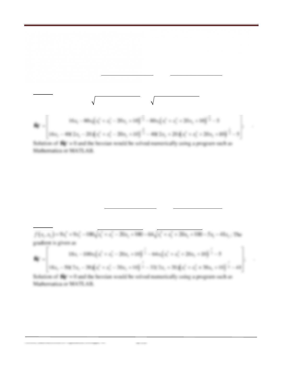
fÑ
= 0 and the hessian would be solved numerically using a program such as
Mathematica or MATLAB.
4.40 ________________________________________________________________________________
Find stationary points for the following function (use a numerical method such as the Newton-
Raphson method, or a software package like Excel, MATLAB, and Mathematica, if needed). Also
determine the local minimum, local maximum, and inflection points for the function (infection
points are those stationary points that are neither minimum nor maximum).
(1,2)= 91
2+ 92
2−100�1
2+2
2−202+100 −64�1
2+2
2+162+64 −51−412
Solution
( )
2 2 22 22
12 1 2 12 2 12 2 1 2
, 9 9 100 20 100 64 20 100 5 41fxx x x xx x xx x x x= + − +− + − ++ + − −
; The
gradient is given as
( ) ( )
( ) ( )
11
22 22
22
1 11 2 2 11 2 2
11
22 22
22
2 2 12 2 2 12 2
18 100 20 10 64 20 10 5
;
18 50 2 20 20 10 32 2 20 20 10 41
x xx x x xx x x
f
x x xx x x xx x
−−
−−
− +− + − ++ + −
=
− − +− + − + ++ + −
() ()
Ñ
.
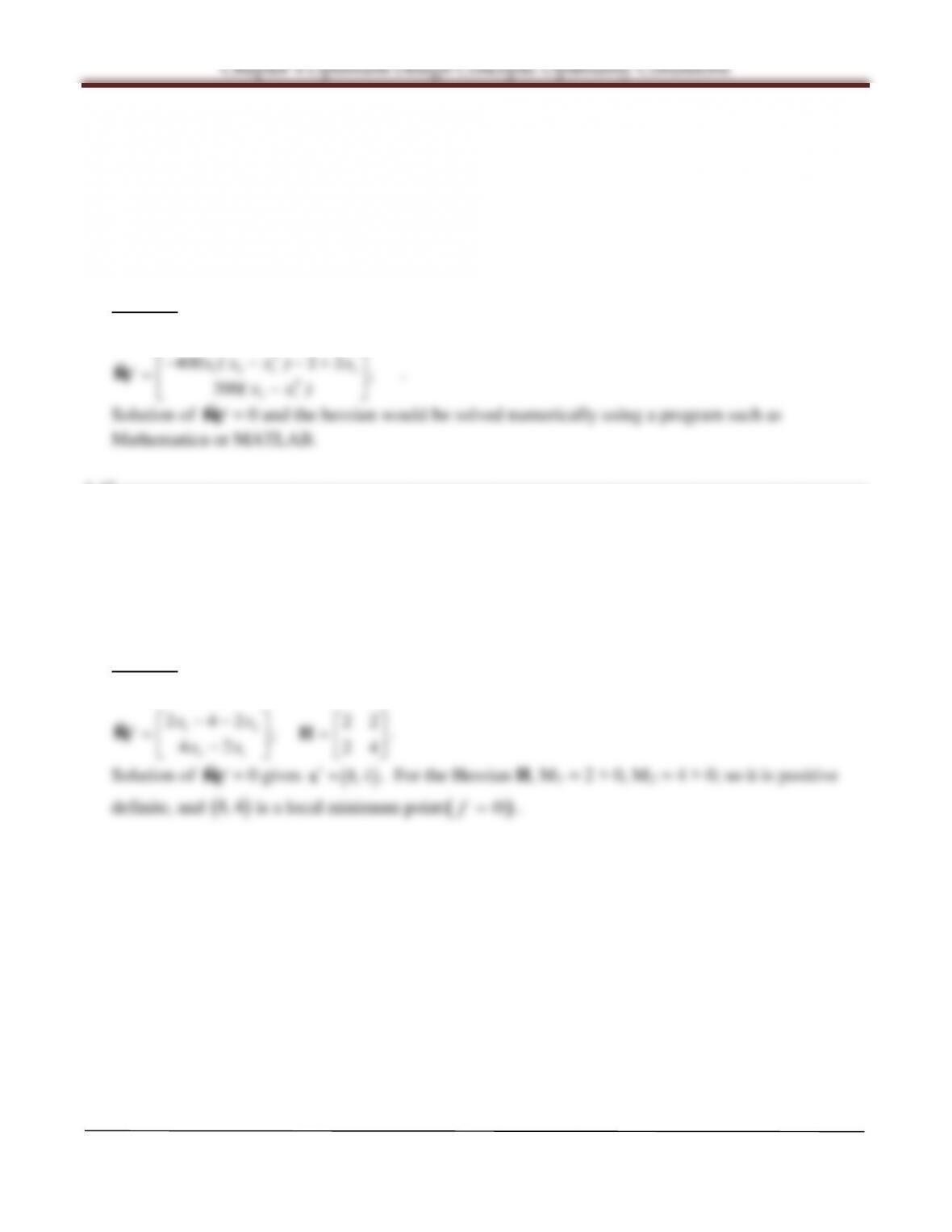
Solution of
fÑ
= 0 and the hessian would be solved numerically using a program such as
Mathematica or MATLAB.
Arora, Introduction to Optimum Design, 4e
4-20
4.41 ________________________________________________________________________________
Find stationary points for the following function (use a numerical method such as the Newton-
Raphson method, or a software package like Excel, MATLAB, and Mathematica, if needed). Also
determine the local minimum, local maximum, and inflection points for the function (infection
points are those stationary points that are neither minimum nor maximum).
(1,2)=100(2− 1
2)2+ (1 − 1)2
Solution
( )
22 2
12 2 1 1
, 100( ) (1 )fxx x x x= − +−
; The gradient is given as
2
12 1 1
2
21
400 2 2 ;
200
xx x x
fxx
− − −+
=
−
()
()
Ñ
.
Solution of
fÑ
= 0 and the hessian would be solved numerically using a program such as
Mathematica or MATLAB.
4.42 ________________________________________________________________________________
Find stationary points for the following function (use a numerical method such as the Newton-
Raphson method, or a software package like Excel, MATLAB, and Mathematica, if needed). Also
determine the local minimum, local maximum, and inflection points for the function (infection
points are those stationary points that are neither minimum nor maximum).
(1,2,3,4)=(1−102)2+ 5(3− 4)2+(2−23)4+10(1− 4)4
Solution
( )
224 4
1234 1 2 3 4 2 3 1 4
, , , ( 10 ) 5( ) ( 2 ) 10( )fxxxx x x x x x x x x=− + − +− + −
; The gradient is given as
12
21
2 42 22
;
42 24
xx
fxx
−−
= =
−
HÑ
.
Solution of
fÑ
= 0 gives
( )
8, 4
∗
=x
. For the Hessian H, M1 = 2 > 0, M2 = 4 > 0; so it is positive
definite, and
( )
8, 4
is a local minimum point
( )
0f=
.