Chapter 4 Optimum Design Concepts
Referring to Exercise 4.62, the point satisfying the KKT necessary conditions is
SECOND ORDER CONDITIONS ARE DISCUSSED IN CHAPTER 5
(1,2)= 41
2+ 32
2−512−81
The gradient of cost function is
MATLAB Code for Exercise 115
clear all
axis equal
[x1,x2]=meshgrid(0:0.01:4, –1:0.01:4);
b=[1.73913];
plot(a,b,‘.k’);
Chapter 4 Optimum Design Concepts
Arora, Introduction to Optimum Design, 4e
4-138
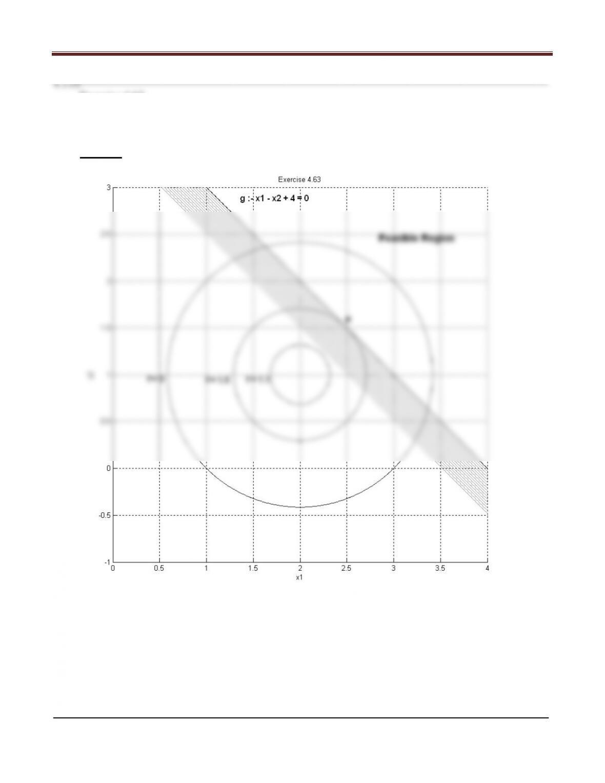
Exercise 4.63
Minimize (1,2)=1
2+2
2−41−22+ 6
subject to 1+2≥4
Solution
Chapter 4 Optimum Design Concepts
Referring to Exercise 4.63, the point satisfying the KKT necessary conditions is
SECOND ORDER CONDITIONS ARE DISCUSSED IN CHAPTER 5
The Hessian of cost function is positive definite, and the constraint function is linear. So, this is a
convex problem. It follows from Theorem 4.11 the point is an isolated global minimum.
2+2
2−41−22+ 6
2(1.5)−2�=�1
1�and ∇g = −�1
1�
We need to check (4.52) from P.131
− ∇f = u∇g
− �1
Chapter 4 Optimum Design Concepts
MATLAB Code for Exercise 116
clear all
axis equal
[x1,x2]=meshgrid(0:0.01:4, –1:0.01:3);
a=[2.5];
b=[1.5];
plot(a,b,‘.k’);
Arora, Introduction to Optimum Design, 4e
4-141
4.117_______________________________________________________________________________
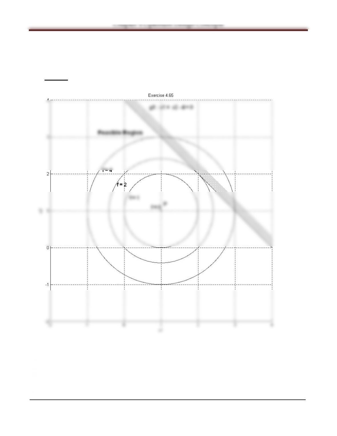
Exercise 4.64
Minimize (1,2)= 21
2−612+ 92
2−181+ 92
subject to 1+ 22≤10
41−32≤20
≥0; = 1,2
Solution
Chapter 4 Optimum Design Concepts
Referring to Exercise 4.64, the point satisfying the KKT necessary conditions is
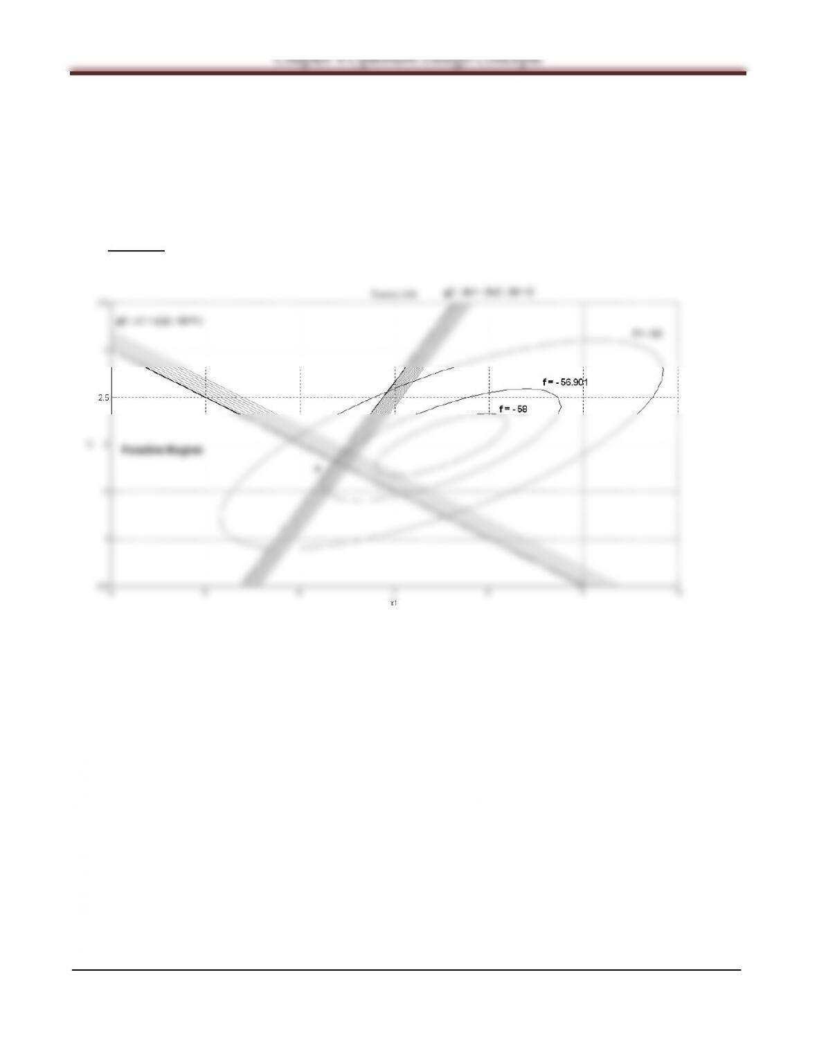
x1= 6.3, x2= 1.733 , u2= 1, f = −56.901
SECOND ORDER CONDITIONS ARE DISCUSSED IN CHAPTER 5
The Hessian of cost function is positive definite, and the constraint function is linear. So, this is a
convex problem. It follows from Theorem 4.11 the point is an isolated global minimum.
The gradient of cost and constraint functions are
At optimum point P (6.3,1.733)
We need to check (4.52) from P.131
which shows local minimum point.
MATLAB Code for Exercise 117
clear all
axis equal
[x1,x2]=meshgrid(4:0.1:10, 0.5:0.1:3.5);
f=2*x1.^2–6*x1.*x2+9*x2.^2–18*x1+9*x2;
cv1=[0:0.05:0.4];
const1=contour(x1,x2,g1,cv1,‘g’);
cv1=[0 0.01];
const1=contour(x1,x2,g1,cv1,‘k’);
cv2=[0:0.05:0.8];
a=[6.3];
b=[1.733];
plot(a,b,‘.k’);
Arora, Introduction to Optimum Design, 4e
4-144
4.118_______________________________________________________________________________
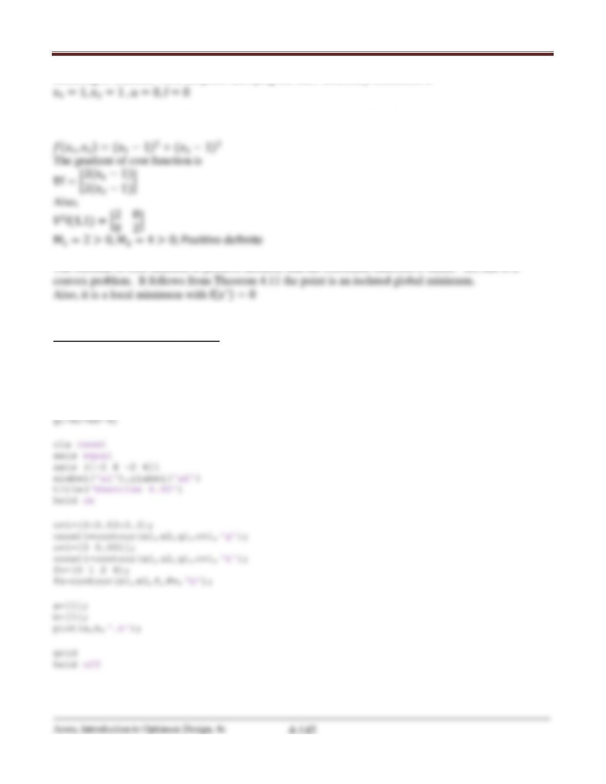
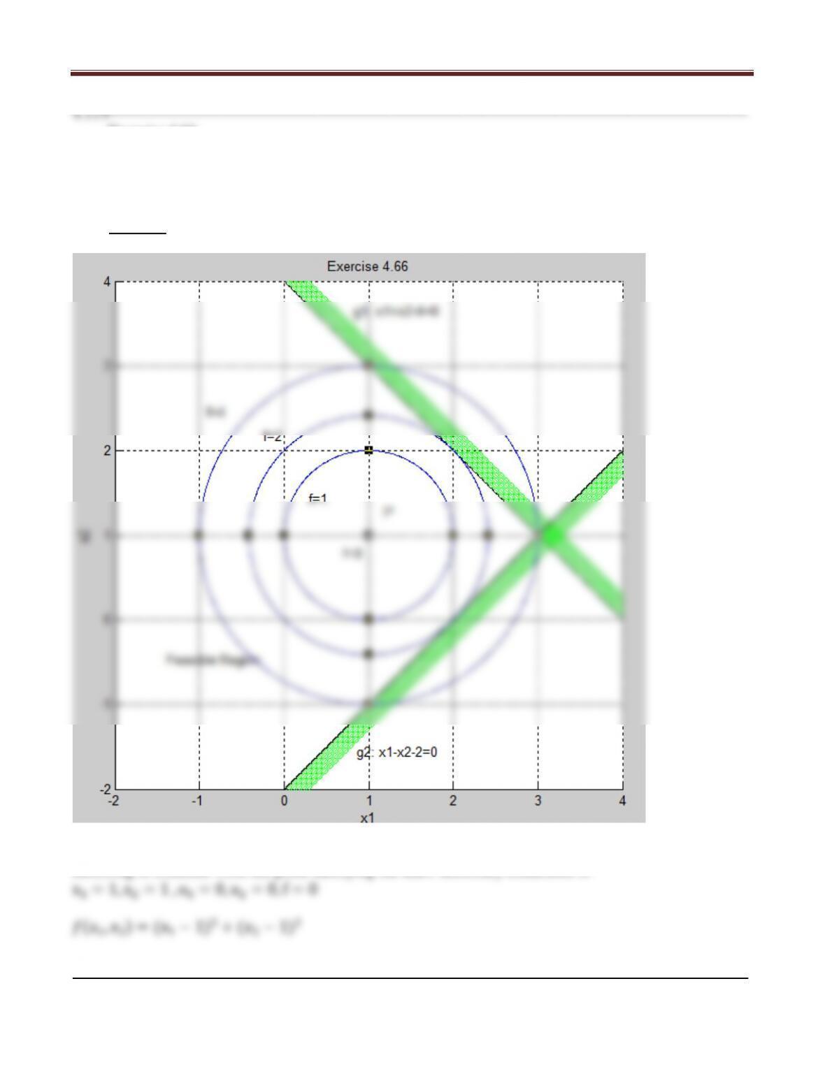
Exercise 4.65 Minimize (1,2)= (1−1)2+ (2−1)2
subject to 1+2−4≤0
Solution
Chapter 4 Optimum Design Concepts
Referring to Exercise 4.65, the point satisfying the KKT necessary conditions is
SECOND ORDER CONDITIONS ARE DISCUSSED IN CHAPTER 5
The Hessian of cost function is positive definite, and the constraint function is linear. So, this is a
MATLAB Code for Exercise 118
clear all
axis equal
[x1,x2]=meshgrid(–2:0.01:4, –2:0.01:4);
f=(x1–1).^2+(x2–1).^2;
Chapter 4 Optimum Design Concepts
Arora, Introduction to Optimum Design, 4e
4-146
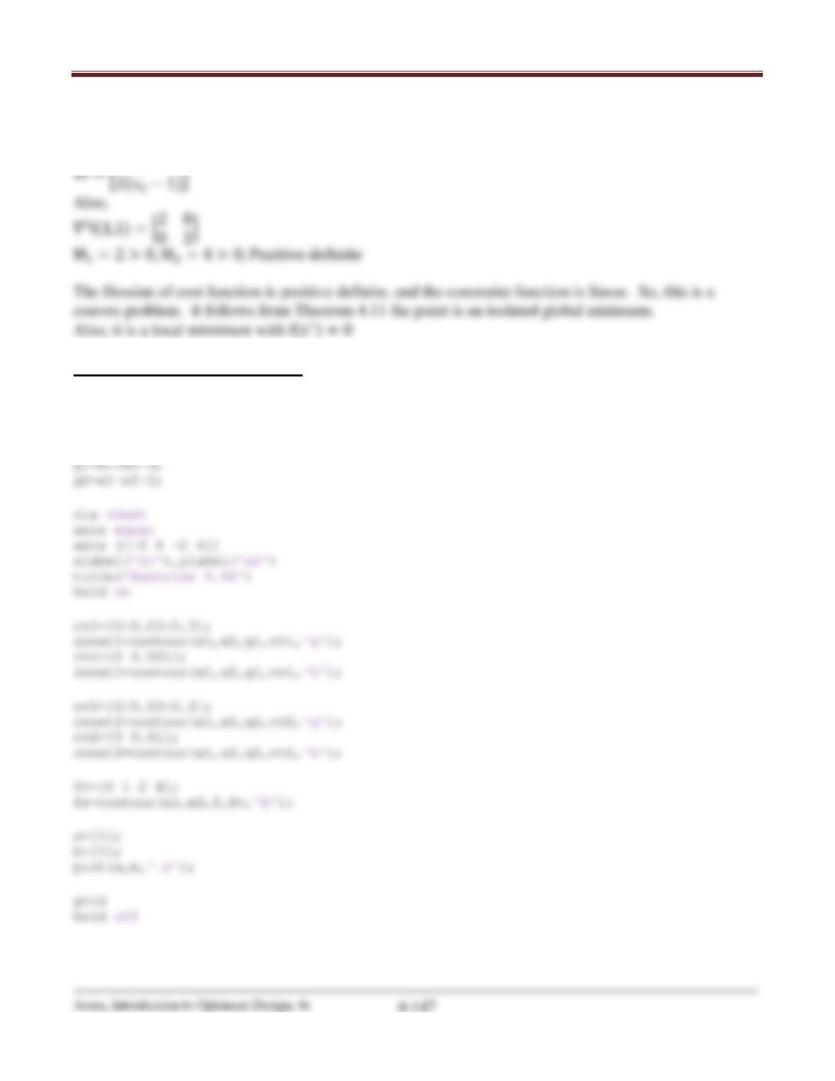
Exercise 4.66
Minimize (1,2)= (1−1)2+ (2−1)2
subject to 1+2−4≤0
1−2−2≤0
Solution
Referring to Exercise 4.66, the point satisfying the KKT necessary conditions is
Chapter 4 Optimum Design Concepts
SECOND ORDER CONDITIONS ARE DISCUSSED IN CHAPTER 5
The gradient of cost function is
MATLAB Code for Exercise 119
clear all
axis equal
[x1,x2]=meshgrid(–2:0.01:4, –2:0.01:4);
f=(x1–1).^2+(x2–1).^2;
Chapter 4 Optimum Design Concepts
Arora, Introduction to Optimum Design, 4e
4-148
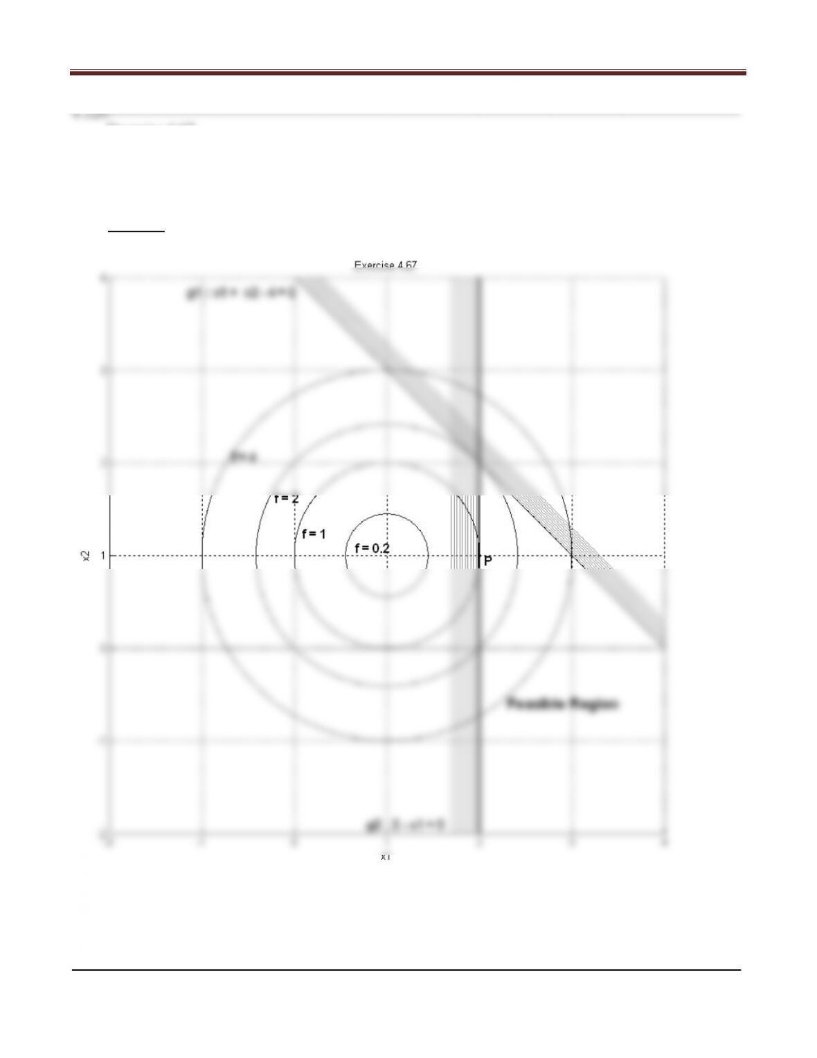
Exercise 4.67
Minimize(1,2)= (1−1)2+ (2−1)2
subject to 1+2−4≤0
2−1≤0
Solution
Chapter 4 Optimum Design Concepts
Arora, Introduction to Optimum Design, 4e
4-149
Referring to Exercise 4.67, the point satisfying the KKT necessary conditions is
x1= 2, x2= 1 , u2= 2, f = 1
SECOND ORDER CONDITIONS ARE DISCUSSED IN CHAPTER 5
The Hessian of cost function is positive definite, and the constraint function is linear. So, this is a
convex problem. It follows from Theorem 4.11 the point is an isolated global minimum.
The gradient of cost and constraint functions are
At optimum point P (2,1)
We need to check (4.52) from P.131
− ∇f = ui∇gi
which shows local minimum point.
By Theorem 4.7,
Chapter 4 Optimum Design Concepts
MATLAB Code for Exercise 120
clear all
axis equal
[x1,x2]=meshgrid(–2:0.01:4, –2:0.01:4);
f=(x1–1).^2+(x2–1).^2;
fv=[0.2 1 2 4];
fs=contour(x1,x2,f,fv,‘b’);
Arora, Introduction to Optimum Design, 4e
4-151
4.121_______________________________________________________________________________
Exercise 4.68
Minimize (1,2)= 91
2−1812+132
2−4
subject to 1
2+2
2+ 21≥16
Solution
Chapter 4 Optimum Design Concepts
We need to find isolated or local minimum point(s) which satisfy both KKT necessary conditions and
sufficient or the second order necessary conditions.
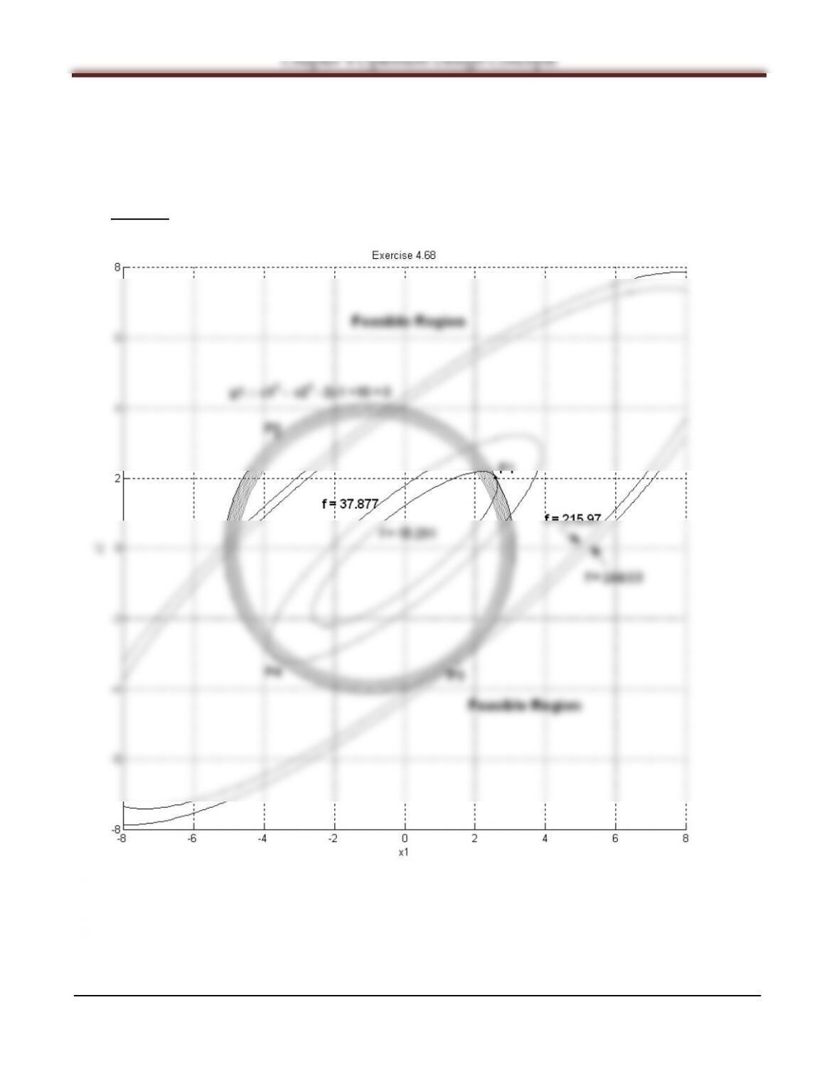
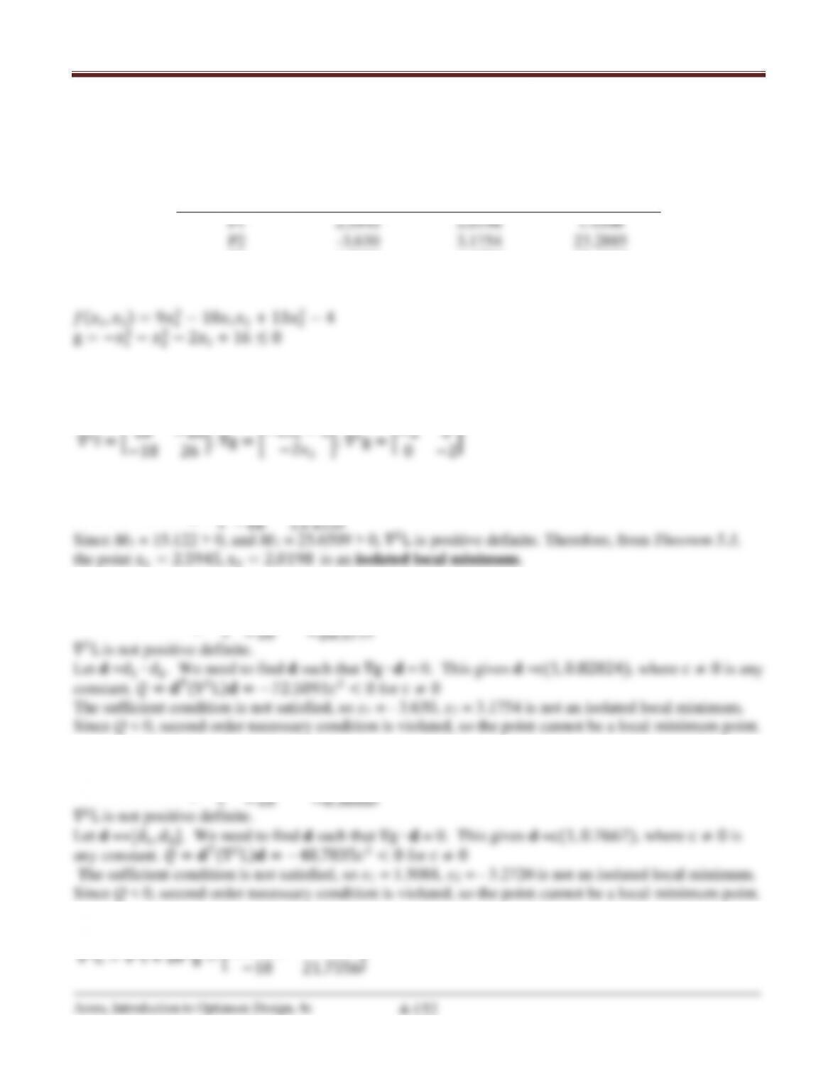
Referring to Exercise 4.68, the points satisfying the KKT necessary conditions are
x1
∗
x2
∗
u1
∗
P1
2.5945
2.0198
1.4390
P2
-3.630
3.1754
23.2885
P3
1.5088
-3.2720
17.1503
P4
-3.7322
-3.0879
2.1222
g = −1
SECOND ORDER CONDITIONS ARE DISCUSSED IN CHAPTER 5
Hessian of cost function, the gradient and Hessian of the constraint are
1. At point P1,
∇2L = ∇2f + u∇2g = �15.122 −18
2. At point P2,
∇2L = ∇2f + u∇2g = �−28.577 −18
3. At point P3,
∇2L = ∇2f + u∇2g = �−16.3006 −18
4. At point P4,
Chapter 4 Optimum Design Concepts
Arora, Introduction to Optimum Design, 4e
4-153
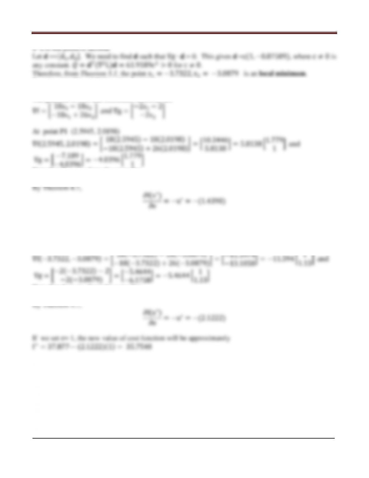
So only point P1 and P4 have local minimum.
The gradient of cost and constraint functions are
Note that they are along the same line.
If we set e = 1, the new value of cost function will be approximately
f∗=15.291— (1.4390)(1)= 13.852
At point P4 (-3.7322, – 3.0879)
Note that they are along the same line.
Chapter 4 Optimum Design Concepts
MATLAB Code for Exercise 121
clear all
axis equal
[x1,x2]=meshgrid(–8:0.1:8, –8:0.1:8);
a=[2.5945 –3.630 1.5088 –3.7322];
b=[2.0198 3.1754 –3.2720 –3.0879];
plot(a,b,‘.k’);
Arora, Introduction to Optimum Design, 4e
4-155
4.122_______________________________________________________________________________
Exercise 4.69
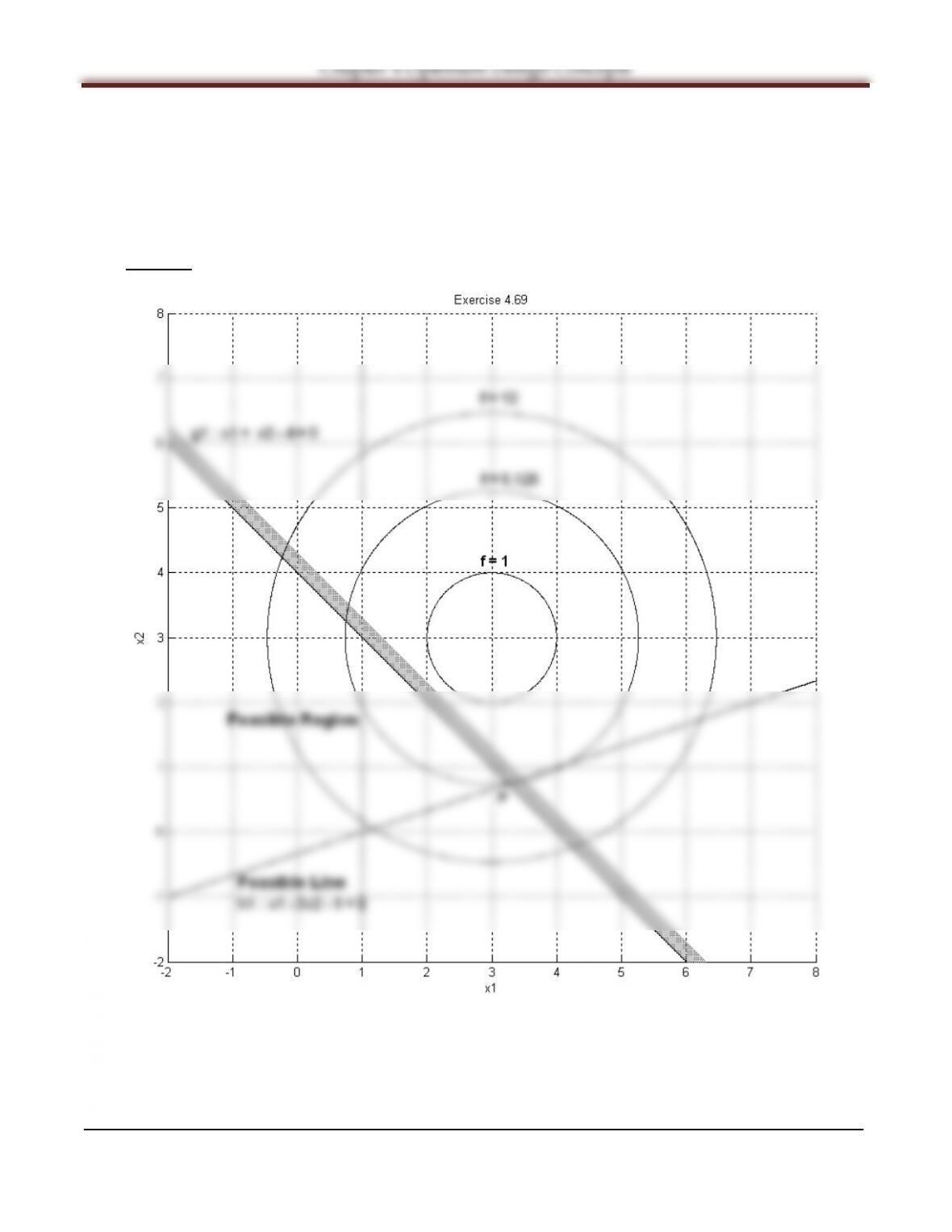
Minimize (1,2)= (1−3)2+ (2−3)2
subject to 1+2≤4
1−32= 1
Solution