Arora, Introduction to Optimum Design, 4e 4-97
4.100_______________________________________________________________________________
Exercise 4.46
Minimize (1,2)= 41
2+ 92
2+ 62−41+13
subject to 1−32+ 3 = 0
Solution
SECOND ORDER CONDITIONS ARE DISCUSSED IN CHAPTER 5
The Hessian of cost function is positive definite, and the constraint function is linear. So, this is a
convex problem. It follows from Theorem 4.11 that the point is an isolated global minimum.
The gradient of cost and constraint functions are
Chapter 4 Optimum Design Concepts
Arora, Introduction to Optimum Design, 4e
4-99
4.101_______________________________________________________________________________
Exercise 4.47
Minimize ()= (1−1)2+ (2+ 2)2+ (3−2)2
subject to 21+ 32−1 = 0
1+2+ 23−4 = 0
Solution
No graphical solution. (3 design variables)
Referring to Exercise 4.47, the point satisfying the KKT necessary conditions is
SECOND ORDER CONDITIONS ARE DISCUSSED IN CHAPTER 5
The Hessian of cost function is positive definite, and the constraint function is linear. So, this is a
convex problem. It follows from Theorem 4.11 the point is an isolated global minimum.
The gradient of cost and constraint functions are
We need to check (4.52) from P.131
which shows local minimum point.
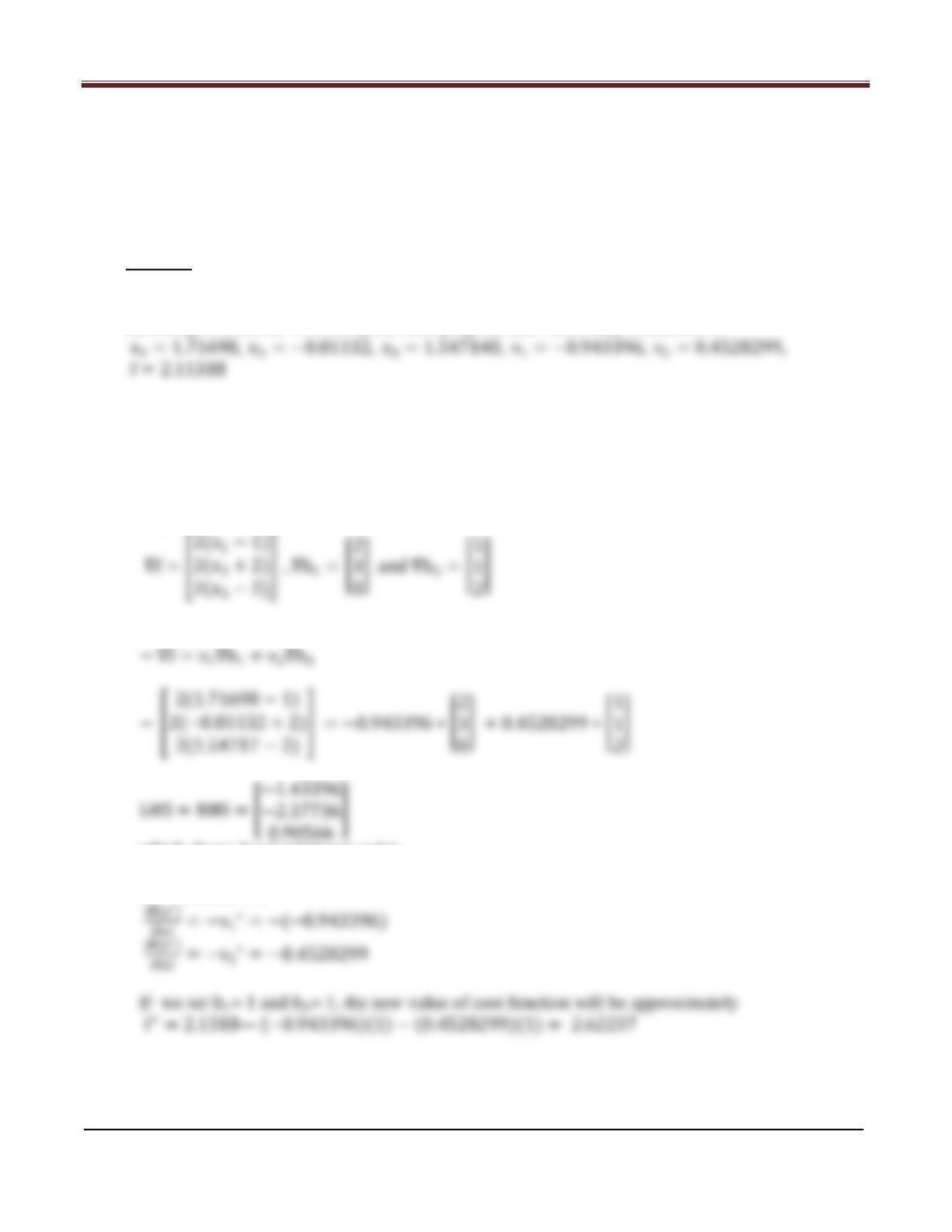
By Theorem 4.7,
Chapter 4 Optimum Design Concepts
Arora, Introduction to Optimum Design, 4e
4-100
4.102_______________________________________________________________________________
Exercise 4.48
Minimize (1,2)= 91
2+1812+132
2−4
subject to 1
2+2
2+ 21=16
Solution
Chapter 4 Optimum Design Concepts
Arora, Introduction to Optimum Design, 4e
4-101
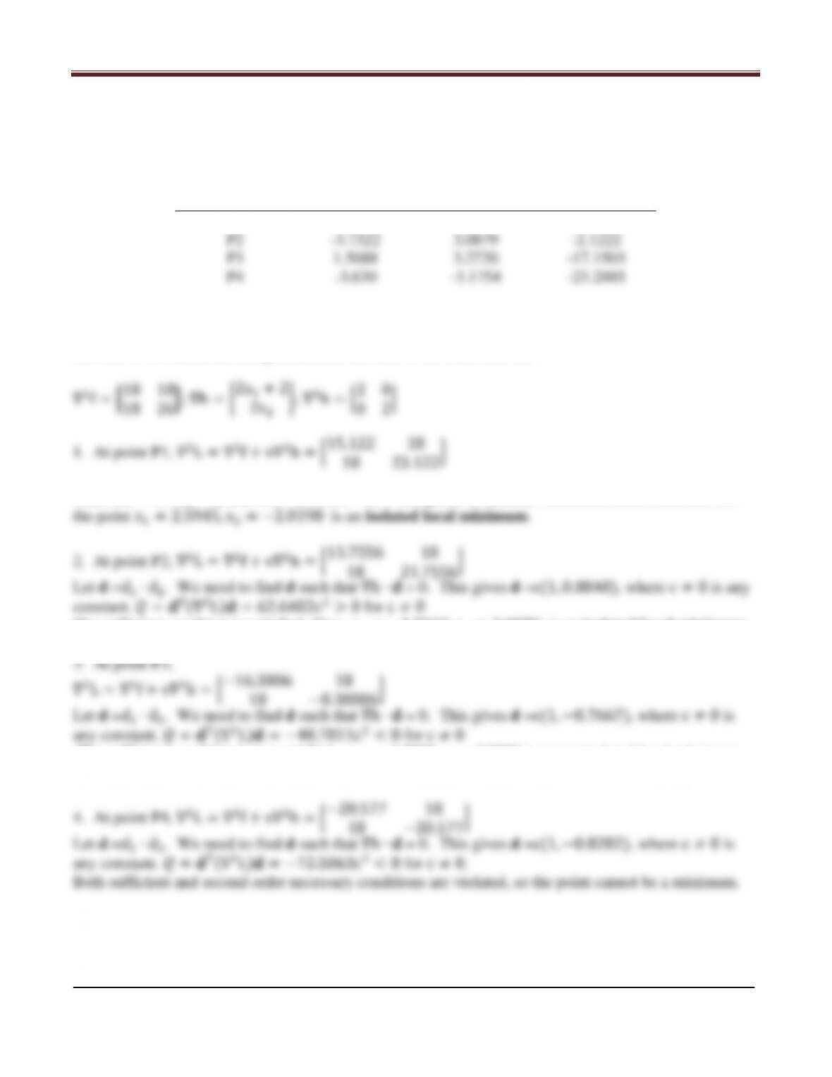
We need to find isolated or local minimum point(s) which satisfy both KKT necessary conditions and
sufficient or the second order necessary conditions.
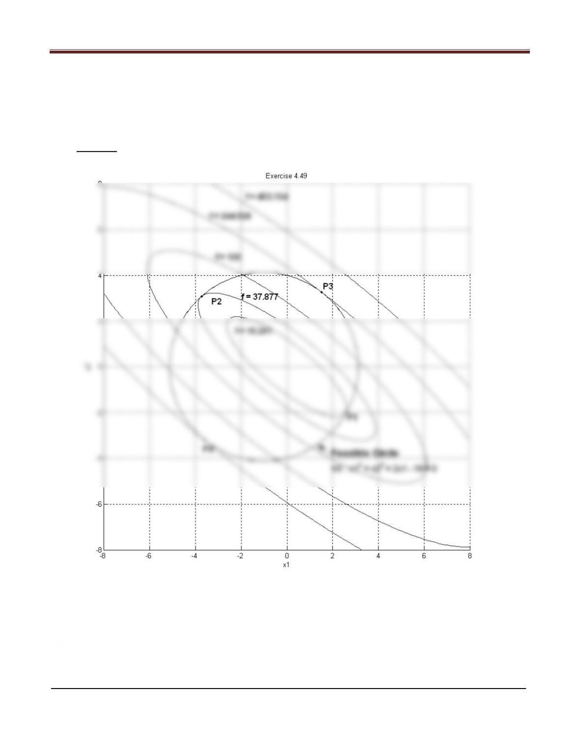
Referring to Exercise 4.48, the points satisfying the KKT necessary conditions are
x1
∗
x2
∗
ν1
∗
P1
2.5945
-2.0198
-1.4390
P2
-3.7322
3.0879
-2.1222
P3
1.5088
3.2720
-17.1503
P4
-3.630
-3.1754
-23.2885
SECOND ORDER CONDITIONS ARE DISCUSSED IN CHAPTER 5
Hessian of cost function, the gradient and Hessian of the constraint are
Since M1 = 15.122 > 0, and M2 = 25.6509 > 0, ∇2L is positive definite. Therefore, from Theorem 5.3,
The sufficient condition is satisfied. Thus, x1=−3.7322, x2= 3.0879 is an isolated local minimum.
The sufficient condition is not satisfied, so x1 = 1.5088, x2 = 3.2720 is not an isolated local minimum.
Since Q < 0, second order necessary condition is violated, so the point cannot be a minimum point.
So only point P1 and P2 have isolated local minimum.
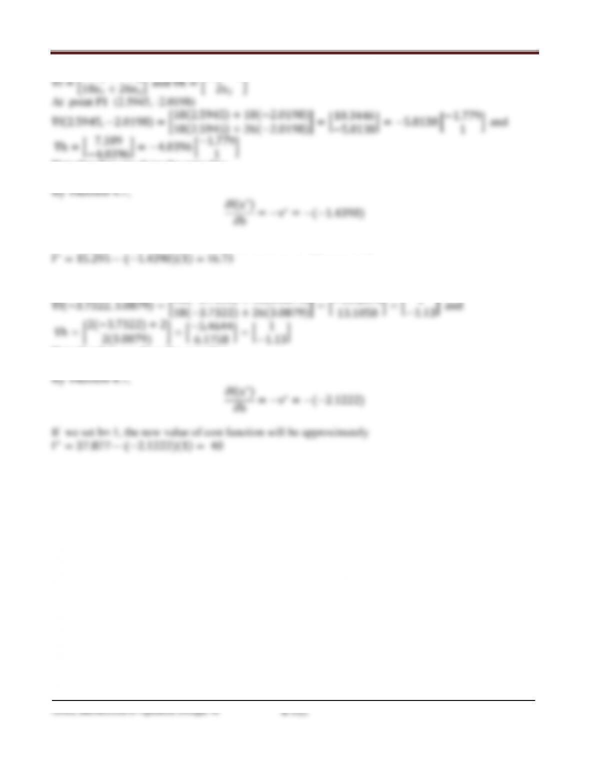
The gradient of cost and constraint functions are
Chapter 4 Optimum Design Concepts
∇f = �18x1+18x2
18x1+26x2� and ∇h = �2x1+ 2
2x2�
At point P1 (2.5945, -2.0198)
∇f(2.5945,−2.0198)=�18(2.5945)+18(−2.0198)
18(2.5945)+26(−2.0198)�=�10.3446
−5.8138�=−5.8138 �−1.779
1� and
∇h = �7.189
−4.0396�=−4.0396 �−1.779
1�
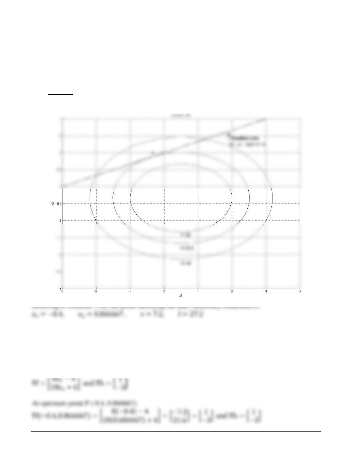
Note that they are along the same line.
If we set b1= 1, the new value of cost function will be approximately
At point P2 (-3.7322, 3.0879)
Note that they are along the same line.
MATLAB Code for Exercise 4.102
clear all
axis equal
[x1,x2]=meshgrid(–8:0.1:8, –8:0.1:8);
fv=[15.291 37.877 100 244.528 453.154];
fs=contour(x1,x2,f,fv,‘b’);
b=[3.2720 –2.0198 –3.1754 3.0879 1.57693 –0.950153];
plot(a,b,‘.k’);
Chapter 4 Optimum Design Concepts
Arora, Introduction to Optimum Design, 4e
4-104
4.103_______________________________________________________________________________
Exercise 4.49
Minimize (1,2)= (1−1)2+ (2−1)2
subject to 1+2−4 = 0
Solution
SECOND ORDER CONDITIONS ARE DISCUSSED IN CHAPTER 5
The Hessian of cost function is positive definite, and the constraint function is linear. So, this is a
convex problem. It follows from Theorem 4.11 the point is an isolated global minimum.
Chapter 4 Optimum Design Concepts
The gradient of cost and constraint functions are
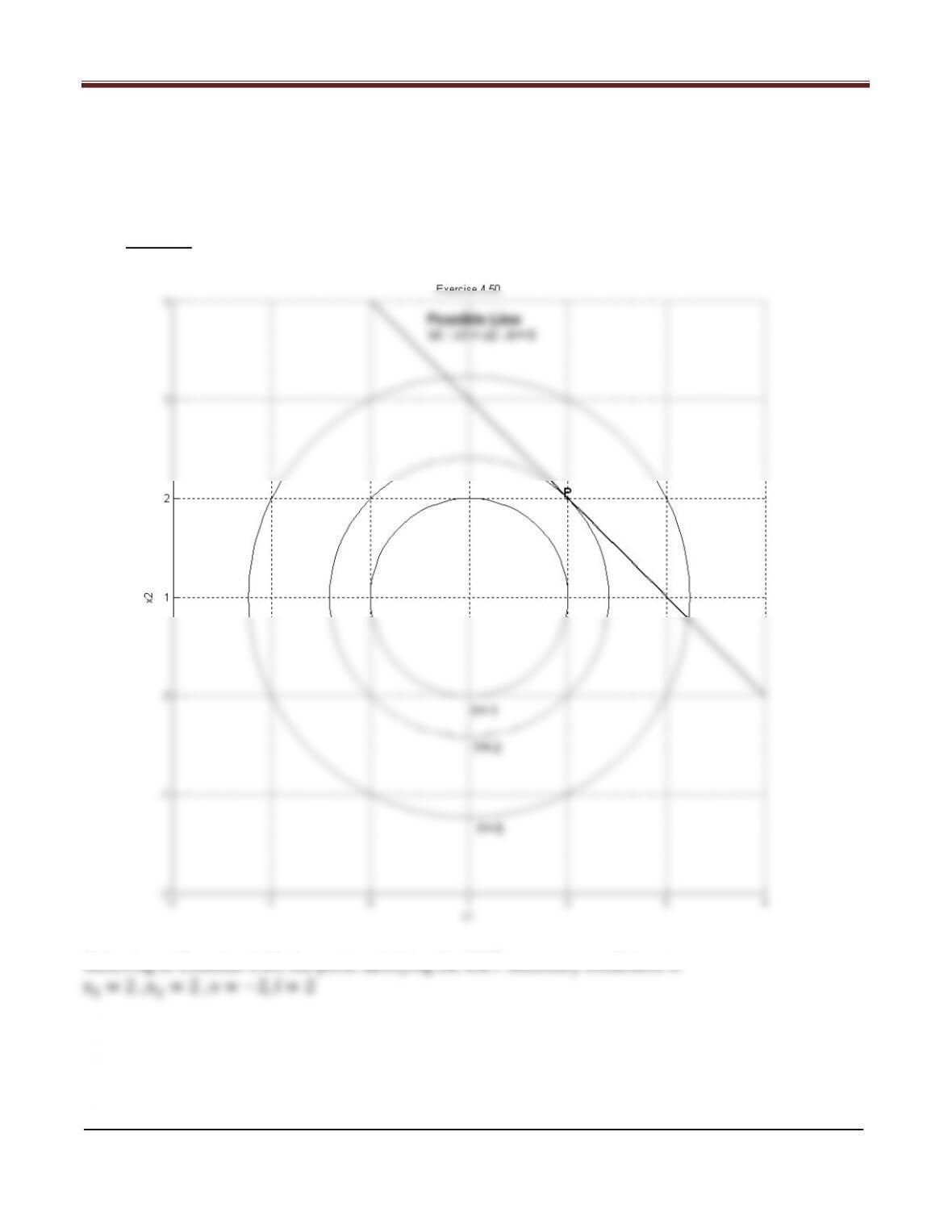
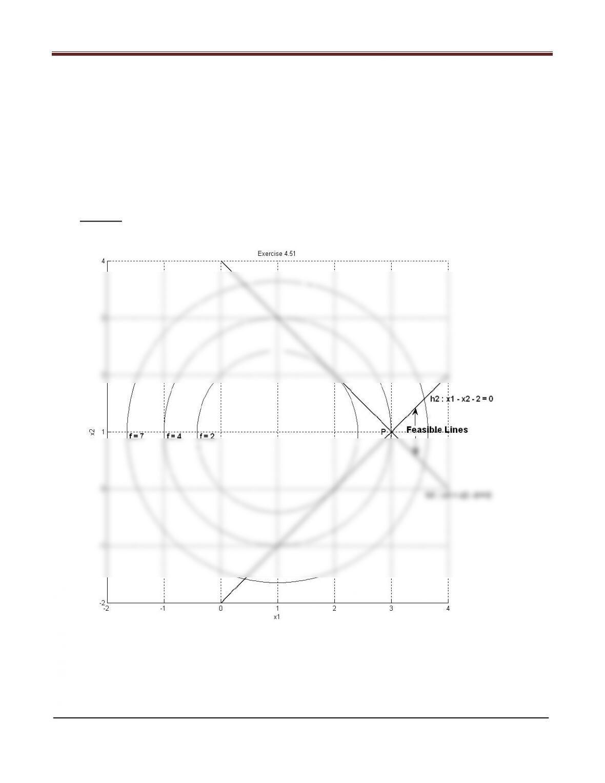
These vectors can be shown at point P in above figure. Note that they will be along the same line.
MATLAB Code for Exercise 4.103
clear all
axis equal
[x1,x2]=meshgrid(–2:0.1:4, –2:0.1:4);
f=(x1–1).^2+(x2–1).^2;
Chapter 4 Optimum Design Concepts
Arora, Introduction to Optimum Design, 4e
4-106
4.104 _______________________________________________________________________________
Exercise 4.50
Consider the following problem with equality constraints:
Minimize (1,2)= (1−1)2+ (2−1)2
subject to 1+2−4 = 0
1−2−2 = 0
1. Is it a valid optimization problem? Explain.
2. Explain how you would solve the problem? Are necessary conditions needed to find the optimum
solution?
Solution
Chapter 4 Optimum Design Concepts
Minimize
( ) ( )
;11 2
2
2
1−+−= xxf
subject to
02 and ,04
2121
=−−=−+ xxxx
(Ref. Exercise 4.50)
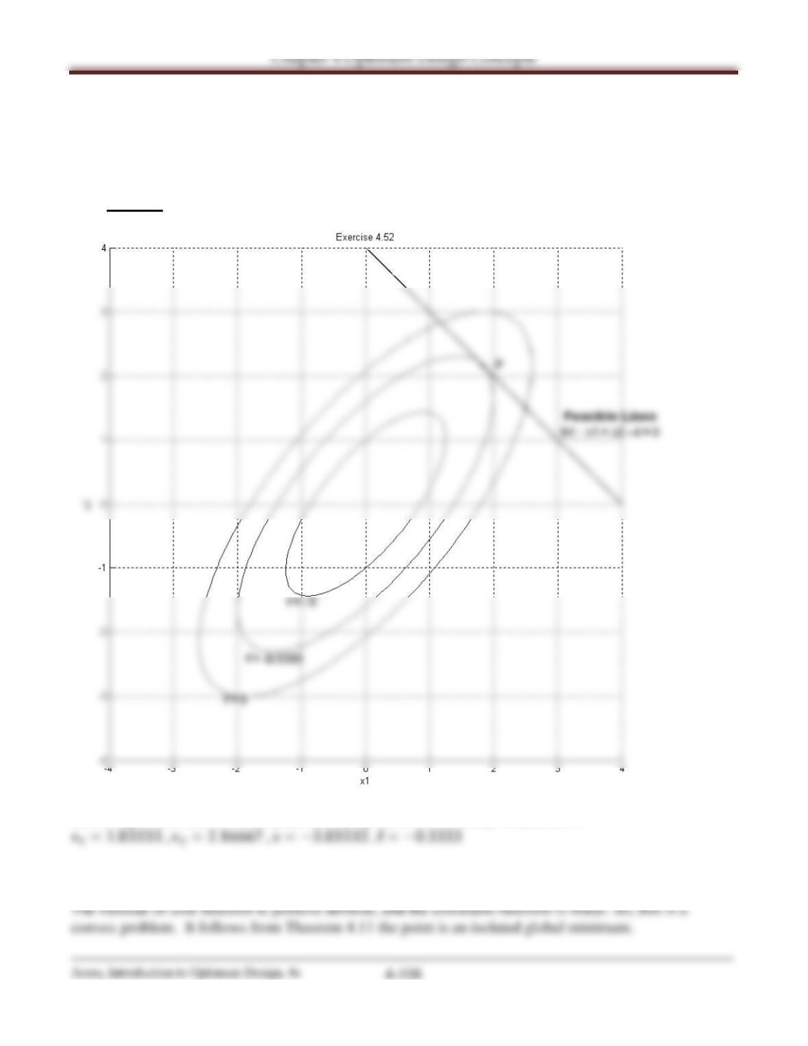
1. It is not a valid optimization problem because there is only one feasible point of the constraint set;
solution of the two linear equalities.
2. Solving the constraint equations, we get x1 = 3, x2 = 1, f (3,1) = 4.
MATLAB Code for Exercise 4.104
clear all
axis equal
[x1,x2]=meshgrid(–2:0.1:4, –2:0.1:4);
f=(x1–1).^2+(x2–1).^2;
4.105_______________________________________________________________________________
Exercise 4.51
Minimize (1,2)= 41
2+ 32
2−512−8
subject to 1+2= 4
Solution
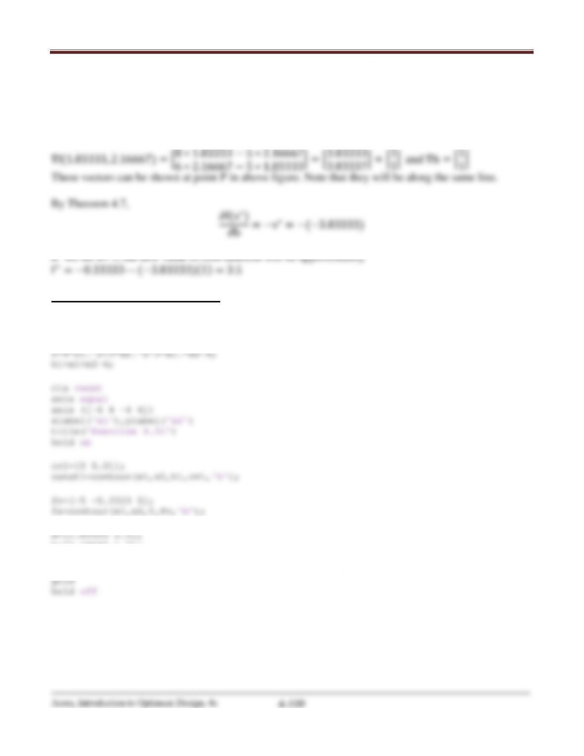
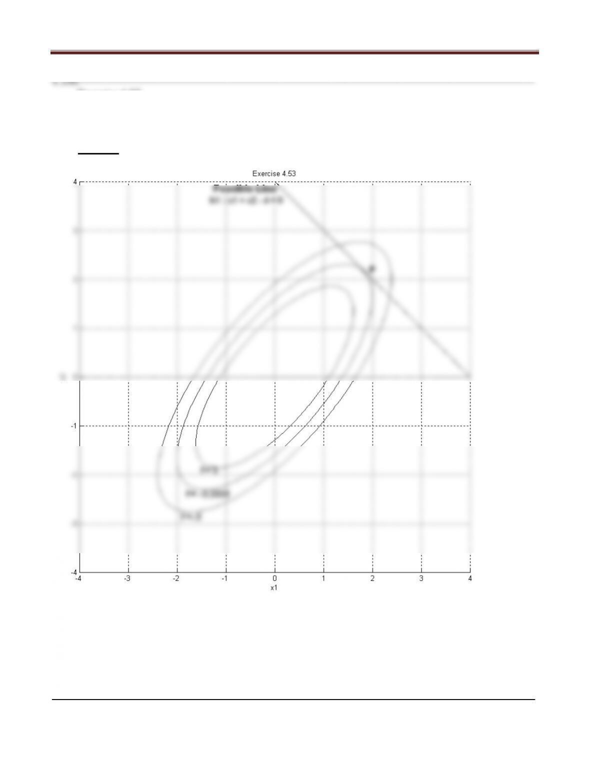
Referring to Exercise 4.51, the point satisfying the KKT necessary conditions is
SECOND ORDER CONDITIONS ARE DISCUSSED IN CHAPTER 5
Chapter 4 Optimum Design Concepts
The gradient of cost and constraint functions are
∇f = �8x1−5x2
6x2−5x1� and ∇h = �1
1�
At optimum point P (1.83333, 2.16667)
MATLAB Code for Exercise 4.105
clear all
axis equal
[x1,x2]=meshgrid(–4:0.1:4, –4:0.1:4);
b=[2.16667 1.5];
plot(a,b,‘.k’);
Chapter 4 Optimum Design Concepts
Arora, Introduction to Optimum Design, 4e
4-110
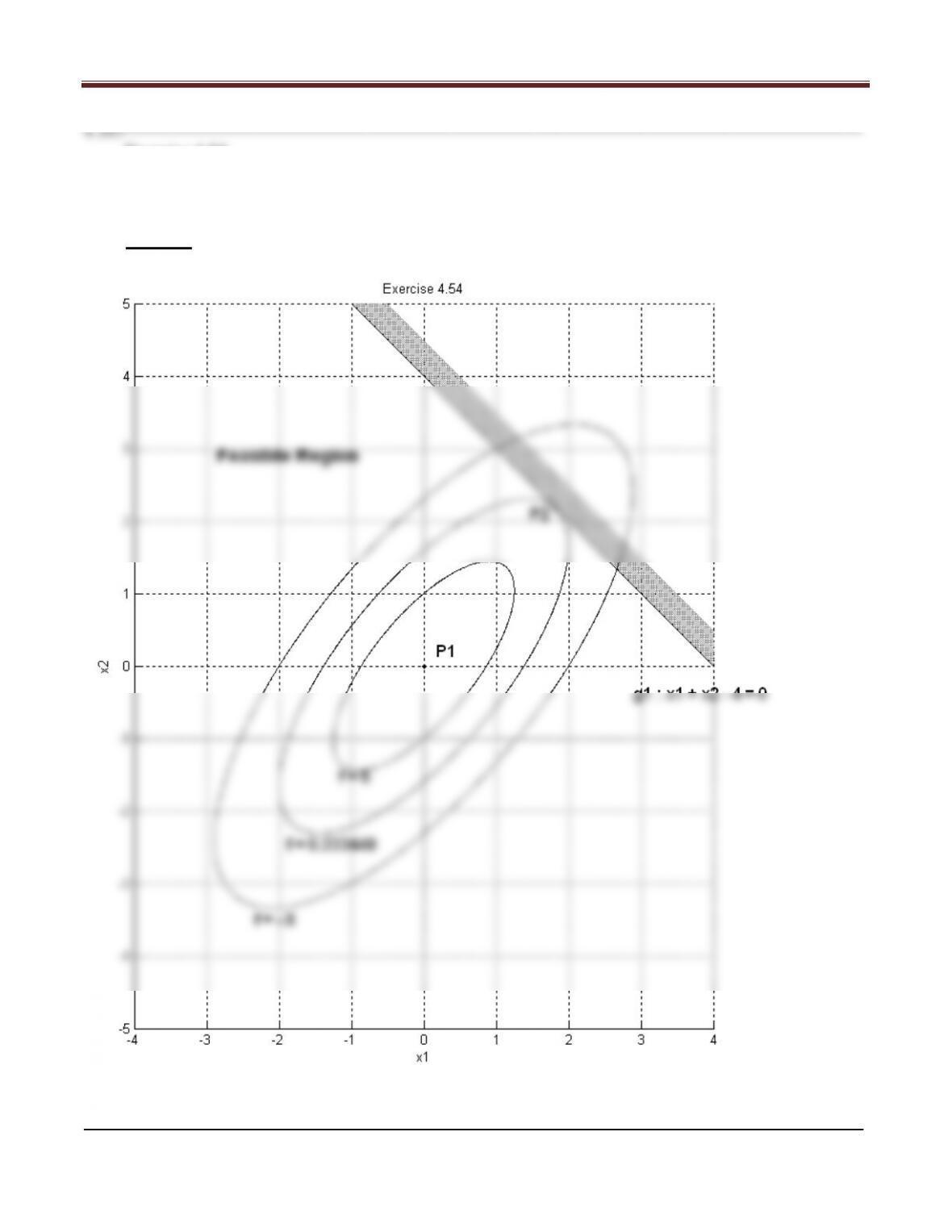
Exercise 4.52
Maximize (1,2)= 41
2+ 32
2−512−8
subject to 1+2= 4
Solution
Chapter 4 Optimum Design Concepts
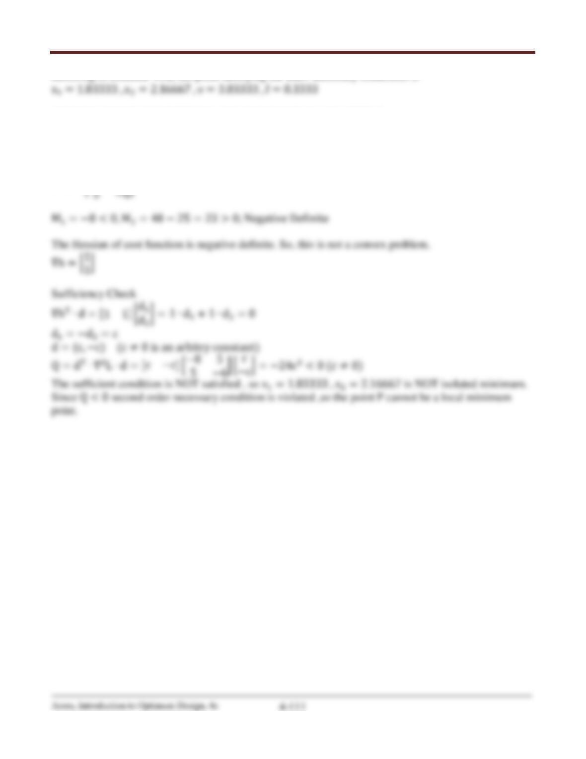
Referring to Exercise 4.52, the point satisfying the KKT necessary conditions is
SECOND ORDER CONDITIONS ARE DISCUSSED IN CHAPTER 5
∇L = �−8x1+ 5x2+ν
−6x2+ 5x1+ν�
∇2L = �−8 5
Chapter 4 Optimum Design Concepts
MATLAB Code for Exercise 4.106
clear all
axis equal
[x1,x2]=meshgrid(–4:0.1:4, –4:0.1:4);
b=[2.16667];
plot(a,b,‘.k’);
Chapter 4 Optimum Design Concepts
Arora, Introduction to Optimum Design, 4e
4-113
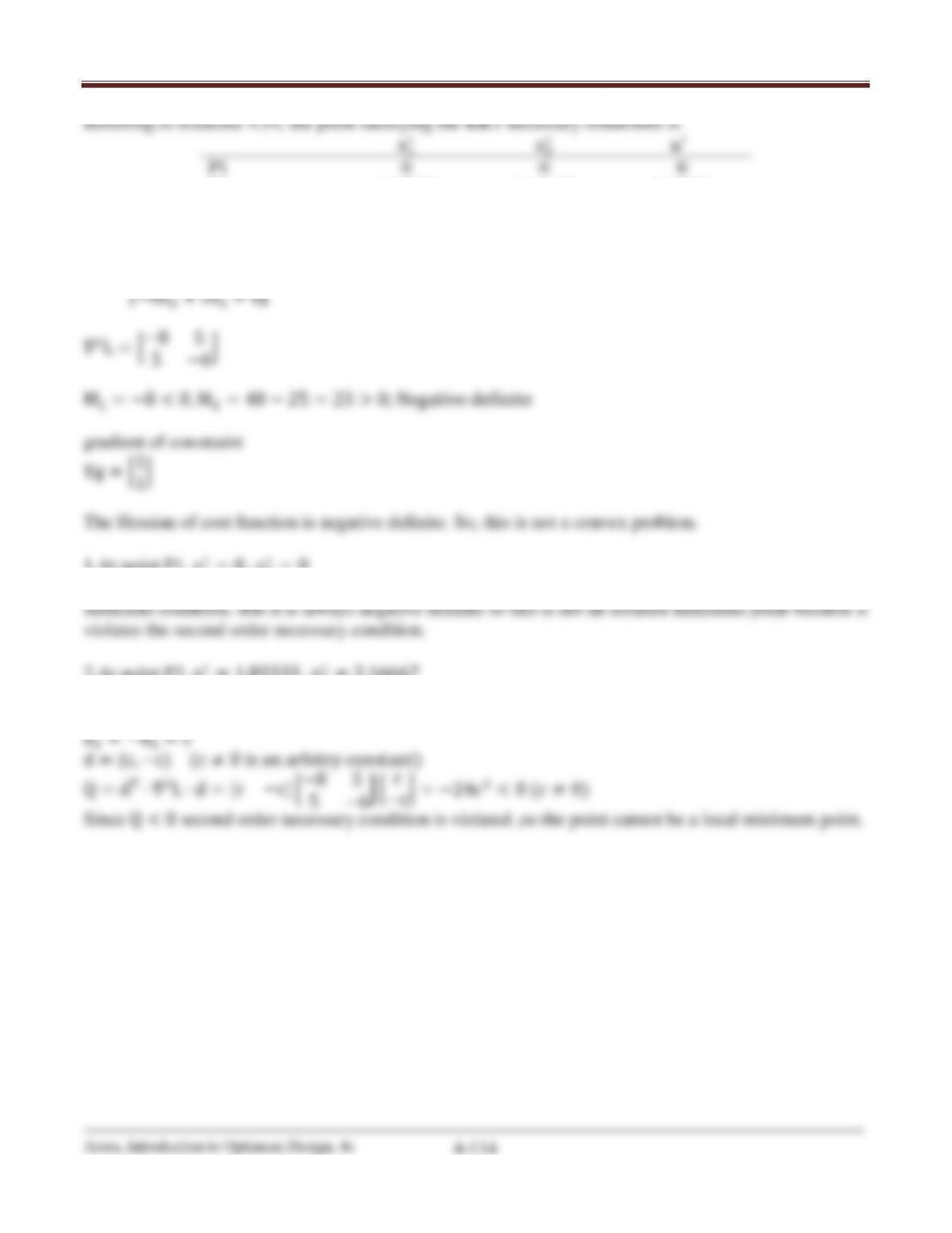
Exercise 4.54
Maximize (1,2)= 41
2+ 32
2−512−8
subject to 1+2≤4
Solution
Chapter 4 Optimum Design Concepts
Referring to Exercise 4.54, the point satisfying the KKT necessary conditions is
x1
∗
x2
∗
u∗
P1
0
0
0
P2
1.83333
2.16667
3.83329
SECOND ORDER CONDITIONS ARE DISCUSSED IN CHAPTER 5
∇L = �−8x1+ 5x2+ u
1.At point P1, x1
Since no constraint is active, Hessian of Lagrangian must be positive definite throughout to satisfy
2.At point P2, x1
∇gT∙d = [1 1]�d1
d2�= 1 ∙d1+ 1 ∙d2= 0
Chapter 4 Optimum Design Concepts
MATLAB Code for Exercise 107
clear all
axis equal
[x1,x2]=meshgrid(–4:0.01:4, –5:0.01:5);
f=(–1)*(4*x1.^2+3*x2.^2–5*x1.*x2–8);
4.108_______________________________________________________________________________
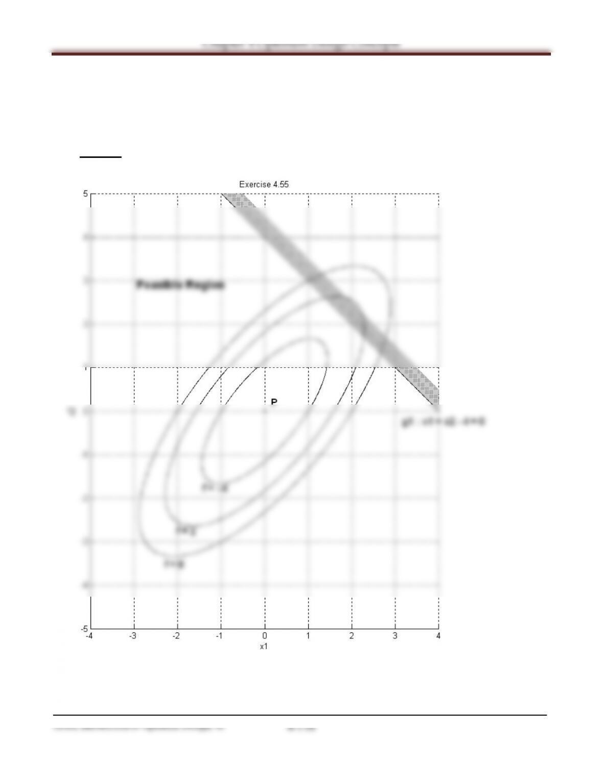
Exercise 4.55
Minimize (1,2)= 41
2+ 32
2−512−8
subject to 1+2≤4
Solution