Chapter 4 Optimum Design Concepts
Arora, Introduction to Optimum Design, 4e
4-117
Referring to Exercise 4.55, the point satisfying the KKT necessary conditions is
SECOND ORDER CONDITIONS ARE DISCUSSED IN CHAPTER 5
MATLAB Code for Exercise 108
clear all
axis equal
[x1,x2]=meshgrid(–4:0.01:4, –5:0.01:5);
f=(4*x1.^2+3*x2.^2–5*x1.*x2–8);
cv1=[0:0.03:0.5];
const1=contour(x1,x2,g1,cv1,‘g’);
cv1=[0 0.001];
Chapter 4 Optimum Design Concepts
Arora, Introduction to Optimum Design, 4e
4-118
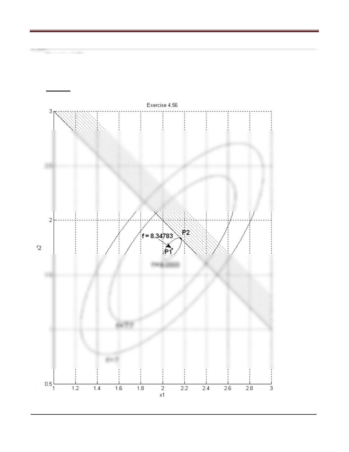
Exercise 4.56
Maximize (1,2)= 41
2+ 32
2−512−81
subject to 1+2≤4
Solution
Chapter 4 Optimum Design Concepts
Arora, Introduction to Optimum Design, 4e
4-119
Referring to Exercise 4.56, the point satisfying the KKT necessary conditions is
x1
∗
x2
∗
u∗
P1
2.08696
1.73913
0
P2
2.16667
1.83333
0.16667
SECOND ORDER CONDITIONS ARE DISCUSSED IN CHAPTER 5
gradient of constraint
∇g = �1
1�
The Hessian of cost function is negative definite. So, this is not a convex problem.
1.At point P1, x1
This is an unconstrained KKT point. The Hessain of the cost function is negative definite, so x1=
2.08696 , x2= 1.73913 is NOT isolated minimum. Actually, the second order necessary condition is
violated, so the point P1 cannot be a local minimum point.
2.At point P2, x1
∗= 2.16667 , x2
∗= 1.83333; ∗= 8.333
Chapter 4 Optimum Design Concepts
MATLAB Code for Exercise 109
clear all
cla reset
axis equal
axis ([–2 4 –2 4])
xlabel(‘x1’),ylabel(‘x2’)
title(‘Exercise 4.56′)
hold on
a=[3];
b=[1];
plot(a,b,‘.k’);
grid
hold off
Arora, Introduction to Optimum Design, 4e
4-121
4.110_______________________________________________________________________________
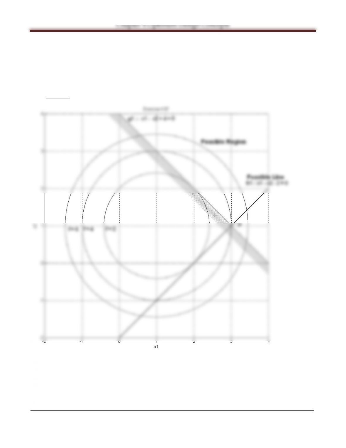
Exercise 4.57
Minimize (1,2)= (1−1)2+ (2−1)2
subject to 1+2≥4
1−2−2 = 0
Solution
Chapter 4 Optimum Design Concepts
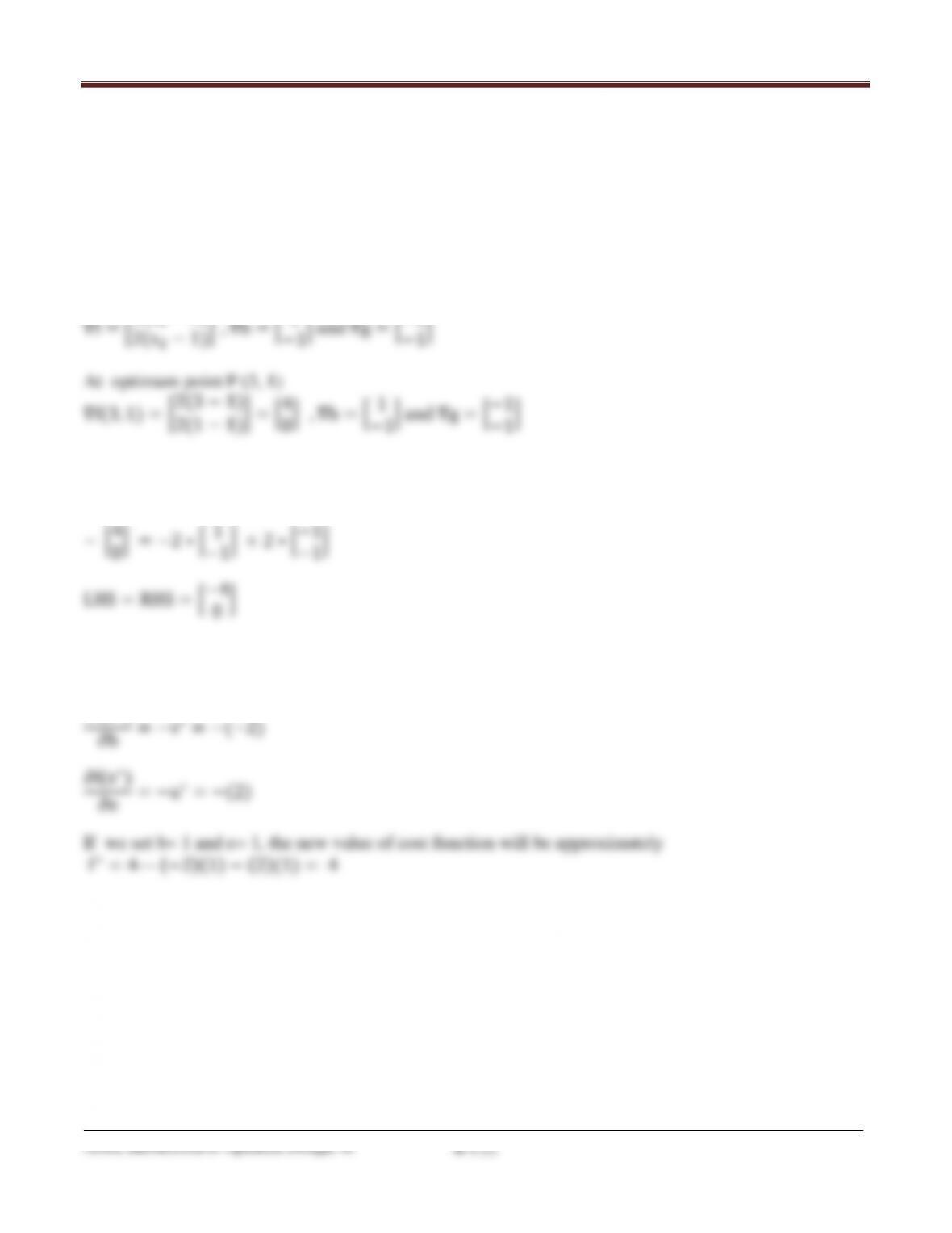
Referring to Exercise 4.57, the point satisfying the KKT necessary conditions is
x1= 3, x2= 1 , ν=−2, u = 2, f = 4
SECOND ORDER CONDITIONS ARE DISCUSSED IN CHAPTER 5
The Hessian of cost function is positive definite, and the constraint function is linear. So, this is a
convex problem. It follows from Theorem 4.11 the point is an isolated global minimum.
The gradient of cost and constraint functions are
We need to check (4.52) from P.131
− ∇f = ν∇h + u∇g
which shows local minimum point.
By Theorem 4.7,
∂f(x∗)
MATLAB Code for Exercise 110
clear all
axis equal
[x1,x2]=meshgrid(–2:0.01:4, –2:0.01:4);
f=(x1–1).^2+(x2–1).^2;
Chapter 4 Optimum Design Concepts
Arora, Introduction to Optimum Design, 4e
4-124
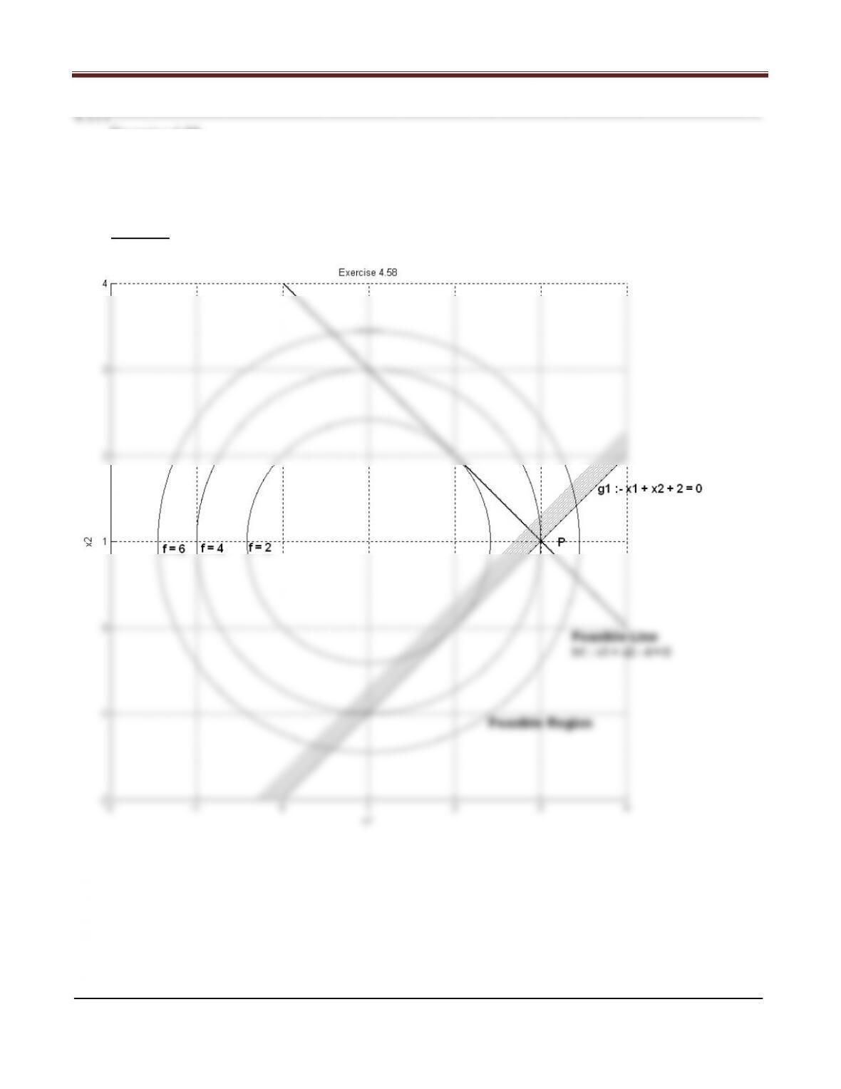
Exercise 4.58
Minimize (1,2)= (1−1)2+ (2−1)2
subject to 1+2= 4
1−2−2≥0
Solution
Chapter 4 Optimum Design Concepts
Arora, Introduction to Optimum Design, 4e
4-125
Referring to Exercise 4.58, the point satisfying the KKT necessary conditions is
SECOND ORDER CONDITIONS ARE DISCUSSED IN CHAPTER 5
The Hessian of cost function is positive definite, and the constraint function is linear. So, this is a
convex problem. It follows from Theorem 4.11 the point is an isolated global minimum.
The gradient of cost and constraint functions are
which shows local minimum point.
By Theorem 4.7,
Chapter 4 Optimum Design Concepts
MATLAB Code for Exercise 111
clear all
cv2=[0 0.01];
const2=contour(x1,x2,h1,cv2,‘k’);
Arora, Introduction to Optimum Design, 4e
4-127
4.112_______________________________________________________________________________
Exercise 4.59
Minimize (1,2)= (1−1)2+ (2−1)2
subject to 1+2≥4
1−2≥2
Solution
Chapter 4 Optimum Design Concepts
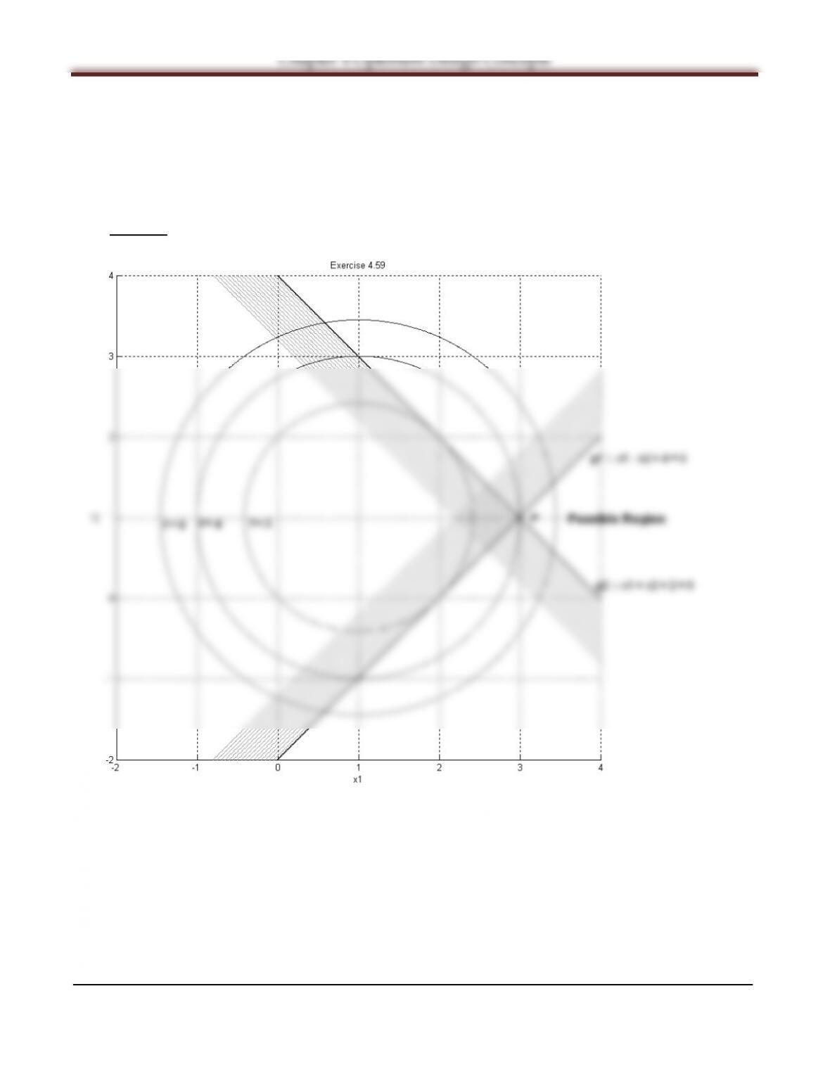
Referring to Exercise 4.59, the point satisfying the KKT necessary conditions is
x1= 3, x2= 1 , u1= 2, u2= 2, f = 4
SECOND ORDER CONDITIONS ARE DISCUSSED IN CHAPTER 5
The Hessian of cost function is positive definite, and the constraint function is linear. So, this is a
convex problem. It follows from Theorem 4.11 the point is an isolated global minimum.
The gradient of cost and constraint functions are
We need to check (4.52) from P.131
− ∇f = u1∇g1+ u2∇g2
which shows local minimum point.
By Theorem 4.7,
Arora, Introduction to Optimum Design, 4e
4-129
MATLAB Code for Exercise 112
clear all
g1=–x1–x2+4;
g2=–x1+x2+2;
cla reset
axis equal
cv1=[0:0.05:0.8];
const1=contour(x1,x2,g1,cv1,‘g’);
cv1=[0 0.01];
const1=contour(x1,x2,g1,cv1,‘k’);
Chapter 4 Optimum Design Concepts
Arora, Introduction to Optimum Design, 4e
4-130
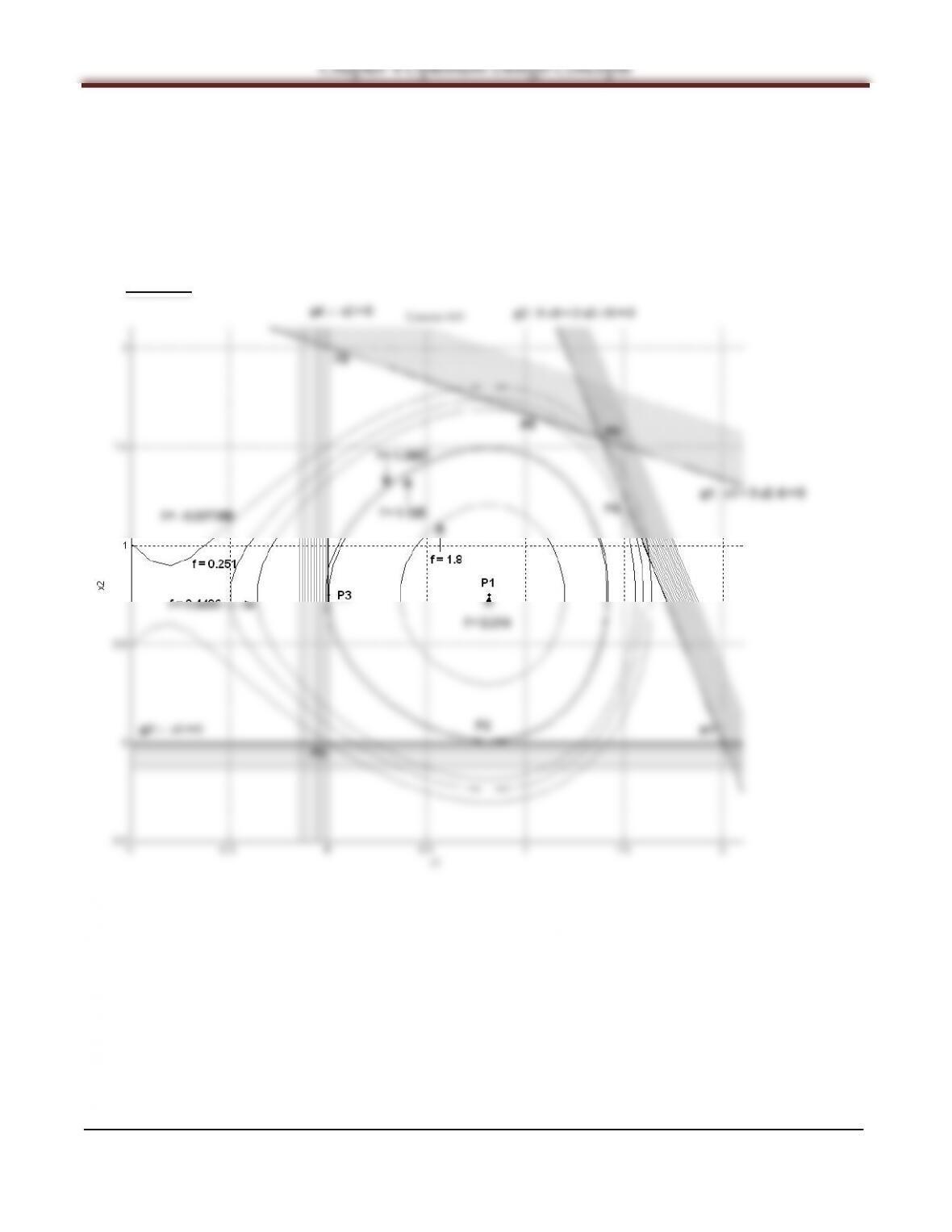
Exercise 4.60
Minimize (,)= (−4)2+ ( −6)2
subject to 12 ≥ +
≥ 6, ≥ 0
Solution
Chapter 4 Optimum Design Concepts
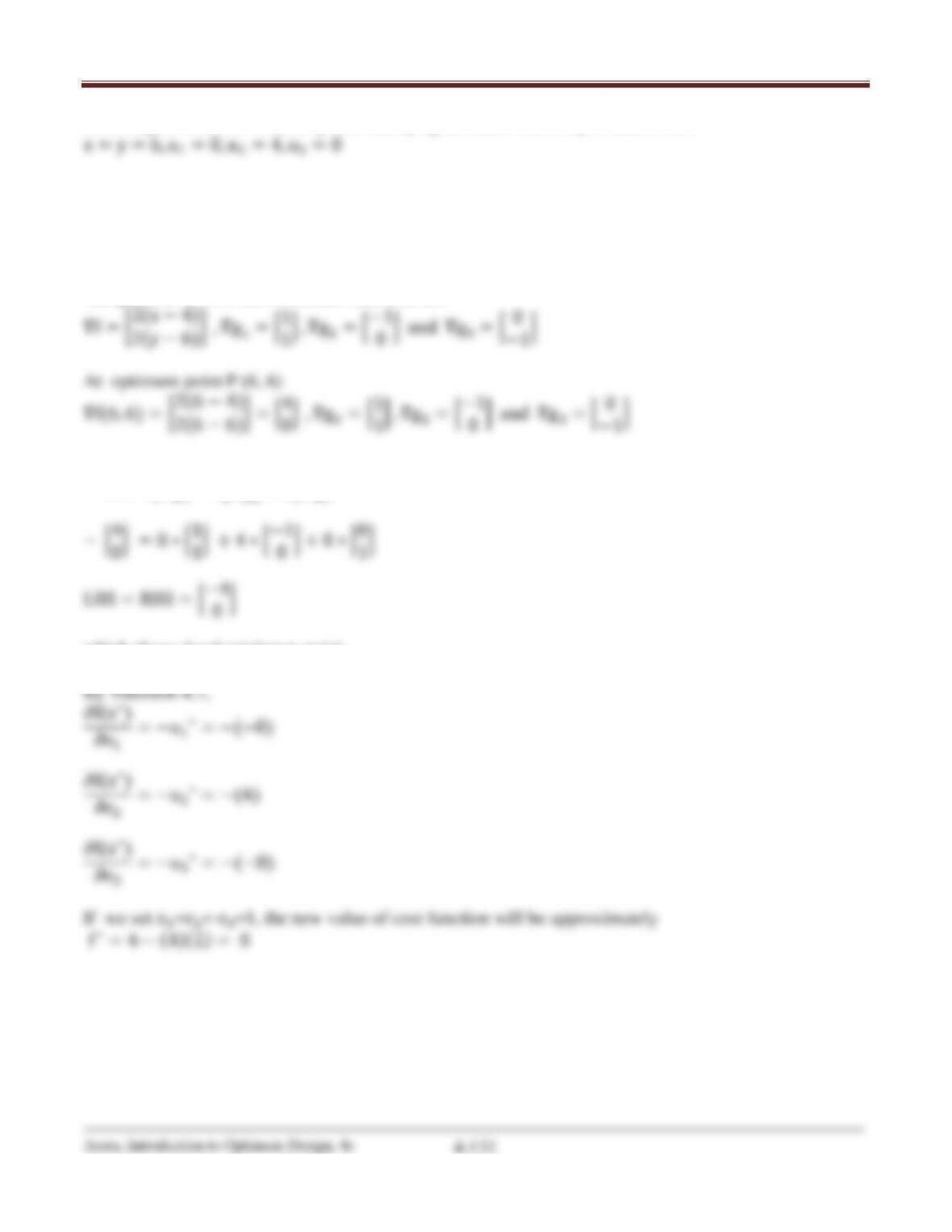
Referring to Exercise 4.60, the points satisfying the KKT necessary conditions are
SECOND ORDER CONDITIONS ARE DISCUSSED IN CHAPTER 5
The Hessian of cost function is positive definite, and the constraint function is linear. So, this is a
convex problem. It follows from Theorem 4.11 the point is an isolated global minimum.
The gradient of cost and constraint functions are
We need to check (4.52) from P.131
− ∇f = u1∇g1+ u2∇g2+ u3∇g3
which shows local minimum point.
Chapter 4 Optimum Design Concepts
MATLAB Code for Exercise 113
clear all
axis equal
[x,y]=meshgrid(–4:0.01:12, –2:0.01:16);
f=(x–4).^2+(y–6).^2;
const1=contour(x,y,g1,cv1,‘g’);
cv1=[0 0.01];
const1=contour(x,y,g1,cv1,‘k’);
cv2=[0:0.05:0.8];
const2=contour(x,y,g2,cv2,‘g’);
Arora, Introduction to Optimum Design, 4e
4-133
4.114_______________________________________________________________________________
Exercise 4.61
Minimize (1,2)= 21+ 32−1
3−22
2
subject to 1+ 32≤6
51+ 22≤10
1,2≥0
Solution
Chapter 4 Optimum Design Concepts
We need to find isolated or local minimum point(s) which satisfy both KKT necessary conditions and
sufficient or the second order necessary conditions.
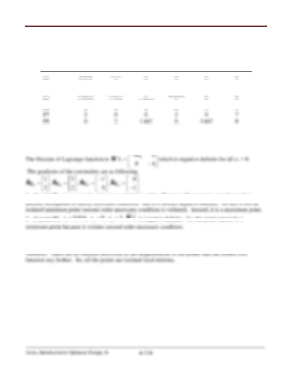
Referring to Exercise 4.61, the points satisfying the KKT necessary conditions are
∗
1
x
∗
2
x
∗
1
u
∗
2
u
∗
3
u
∗
4
u
P1
0.816
0.75
0
0
0
0
P2
0.816
0
0
0
0
3
P3
0
0.75
0
0
2
0
P4
1.5073
1.2317
0
0.9632
0
0
P5
1.0339
1.655
1.2067
0
0
0
P6
0
0
0
0
2
3
P7
2
0
0
2
0
7
P8
0
2
1.667
0
3.667
0
P9
1.386
1.538
0.633
0.626
0
0
SECOND ORDER CONDITIONS ARE DISCUSSED IN CHAPTER 5
1
260
x
12 3 4
32 0 1
−
1. At point P1,
( )
750 ,8130 ..
, since no constraint is active, Hessian of Lagrangian must be positive
2. At point P2,
2
1 24
0.816, 0, 3, x xu L= = = Ñ
is negative definite. So, the point cannot be a
3. For points P3,P4 and P5, since the Hessian of the Lagrangian is negative definite, the three points
cannot be local minima.
4. For points P6,P7,P8 and P9, the number of active constraints is equal to the number of design
MATLAB Code for Exercise 114
clear all
axis equal
[x1,x2]=meshgrid(–1:0.1:2.1, –0.5:0.1:2.1);
f=2*x1+3*x2–x1.^3–2*x2.^2;
cv1=[0:0.05:0.8];
const1=contour(x1,x2,g1,cv1,‘g’);
cv1=[0 0.01];
const1=contour(x1,x2,g1,cv1,‘k’);
cv2=[0:0.05:0.8];
a=[0.816 0.816 0 1.5073 1.0339 0 2 0 1.386 1.28452];
b=[0.75 0 0.75 1.2317 1.655 0 0 2 1.538 0];
plot(a,b,‘.k’);
4.115_______________________________________________________________________________
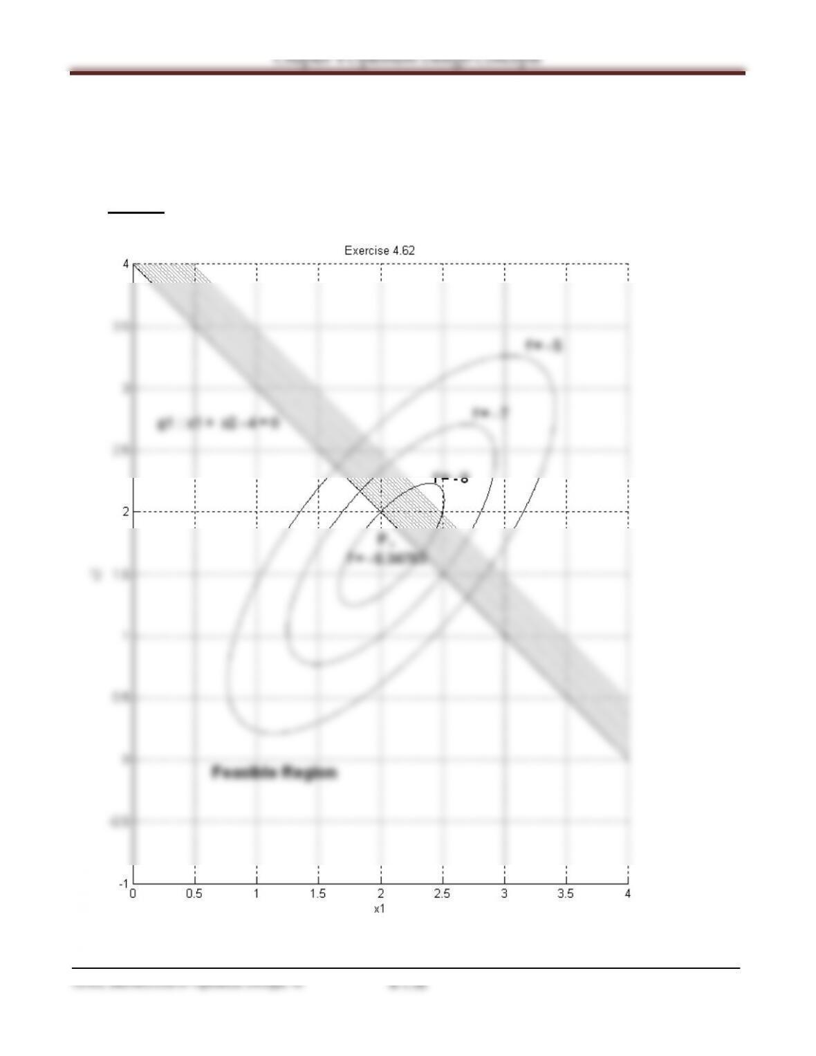
Exercise 4.62
Minimize (1,2)= 41
2+ 32
2−512−81
subject to 1+2≤4
Solution