Arora, Introduction to Optimum Design, 4e
4-76
4.92________________________________________________________________________________
Design a shipping container closed at both ends with dimensions b × b × h to minimize the ratio:
(round-trip cost of shipping the container only) / (one-way cost of shipping the contents only).
Use the following data:
Mass of the container/surface area: 80 kg/ m2
Maximum b: 10 m
Maximum h: 18 m
One-way shipping cost, full of empty :$18/kg gross mass
Mass of the contents: 150 kg/ m3
Formulate the design optimization problem.
Solution
i i ii i
Chapter 4 Optimum Design Concepts: Optimality Conditions
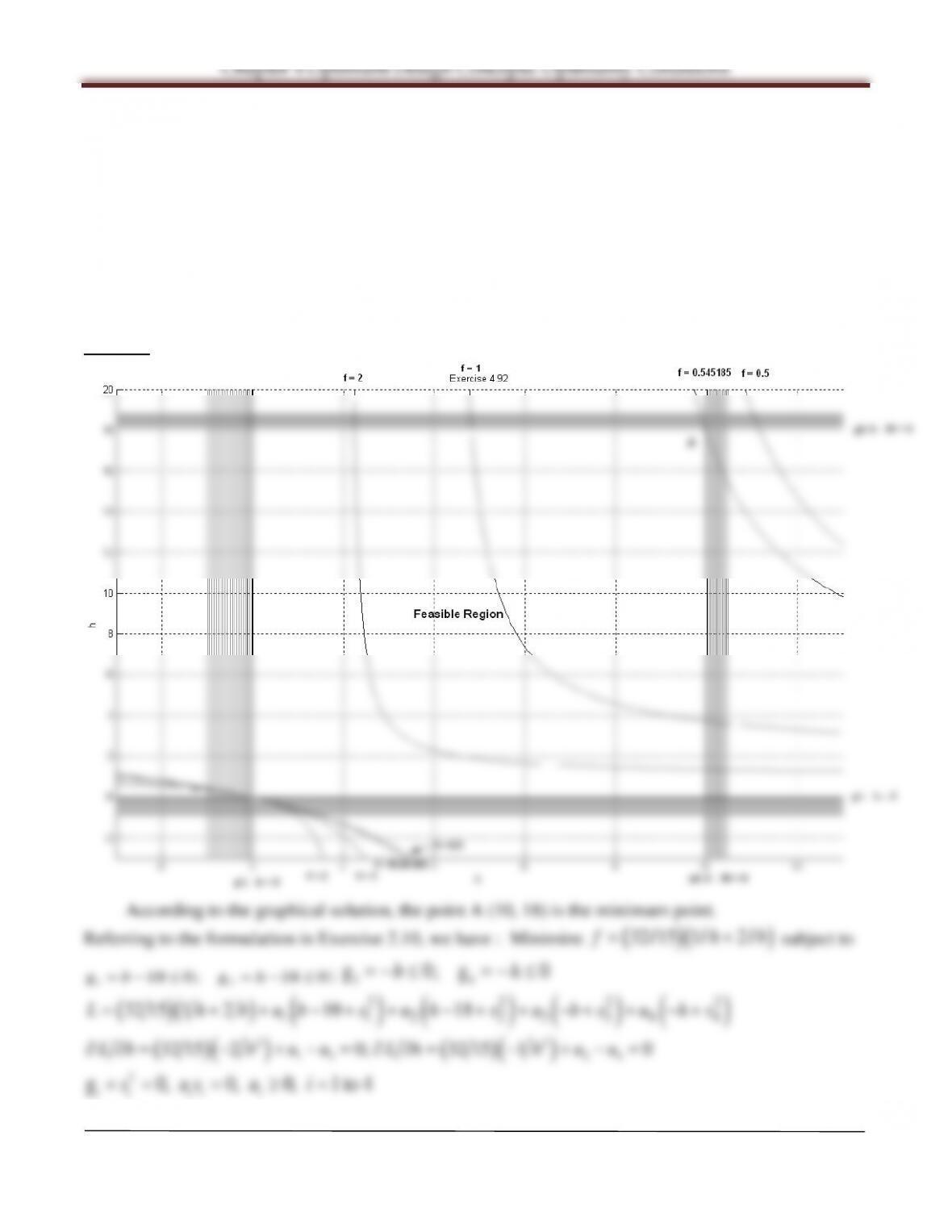
There are 16 cases because there are 4 inequality constraints. The case which yields a solution is given as
0 ,0 2143 ==== ssuu
. The solution is
10, 18,bh= =
12
0 4267, 0 00658,uu= =..
0 545185f=.
. It is
seen from the graph for the problem that the solution is indeed a minimum point and the constraints on
maximum b and h are active.
MATLAB Code for Exercise 4.92
clear all
[b,h]=meshgrid(–3:0.1:15 , –3:0.1:23);
f=(32/15)*(1./h+2./b);
g1=b–10;
cv1=[0:0.03:0.5];
const1=contour(b,h,g1,cv1,‘g’);
cv1=[0 0.001];
const1=contour(b,h,g1,cv1,‘k’);
cv4=[0:0.05:0.9];
const4=contour(b,h,g4,cv4,‘g’);
cv4=[0 0.01];
const4=contour(b,h,g4,cv4,‘k’);
fv=[0.5 0.545185 1 2];
fs=contour(b,h,f,fv,‘b’);
Chapter 4 Optimum Design Concepts: Optimality Conditions
4.93________________________________________________________________________________
Certain mining operations require an open top rectangular container to transport materials. The data
for the problem are:
Construction costs:
sides: $50/m2
ends: $60/m2
bottom: $90/m2
Salvage value: 25 percent of the construction cost
Useful life: 20 years
Yearly maintenance: $12/m2 of outside surface area
Minimum volume needed: 150 m3
Interest rate: 12 percent per annum
Formulate the problem of determining the container dimensions for minimum present cost.
Solution
Referring to the formulation in Exercise 2.11, we have
Design Variables: dimensions of the container; b = width, m; d = depth, m; h = height, m
Cost Function: minimize total present cost;
( ) ( ) ( ) ( )
( )
2 50 2 60 90 1 0.25 0.12, 20
dh bh bd sppwf
++ −
4.94 ________________________________________________________________________________
Design a circular tank closed at both ends to have a volume of 250 m3. The fabrication cost in
proportional to the surface area of the sheet metal and is $400/m2. The tank is to be housed in a shed
with a sloping roof. Therefore, height H of the tank is limited by the relation H ≤ 10 – D/2, where D
is the diameter of the tank. Formulate the minimum cost design problem.
Solution
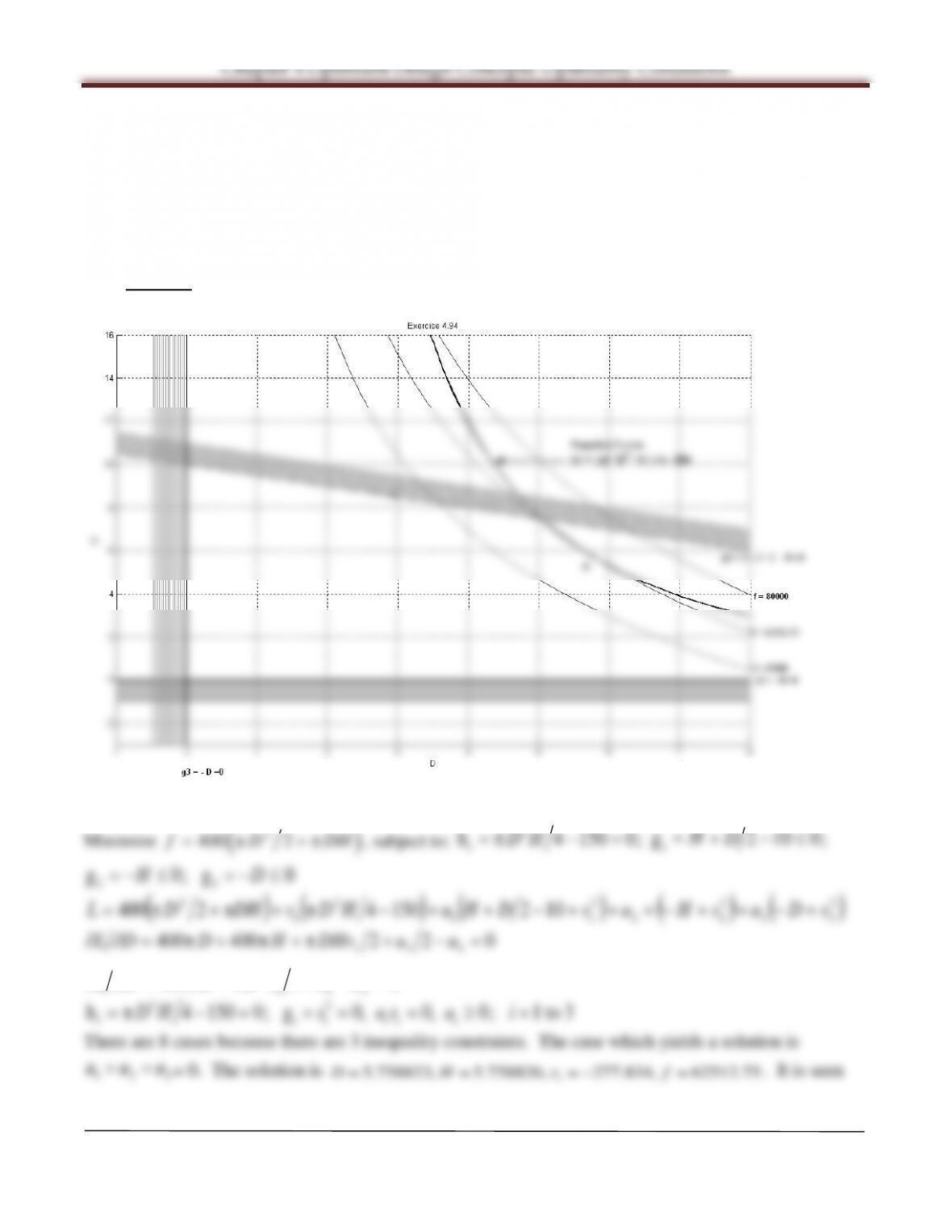
According to the graphical solution, the point A (5.758823, 5.758826) is minimum point.
Referring to the formulation in Exercise 2.12, we have
2
2
Arora, Introduction to Optimum Design, 4e
4-81
4.95________________________________________________________________________________
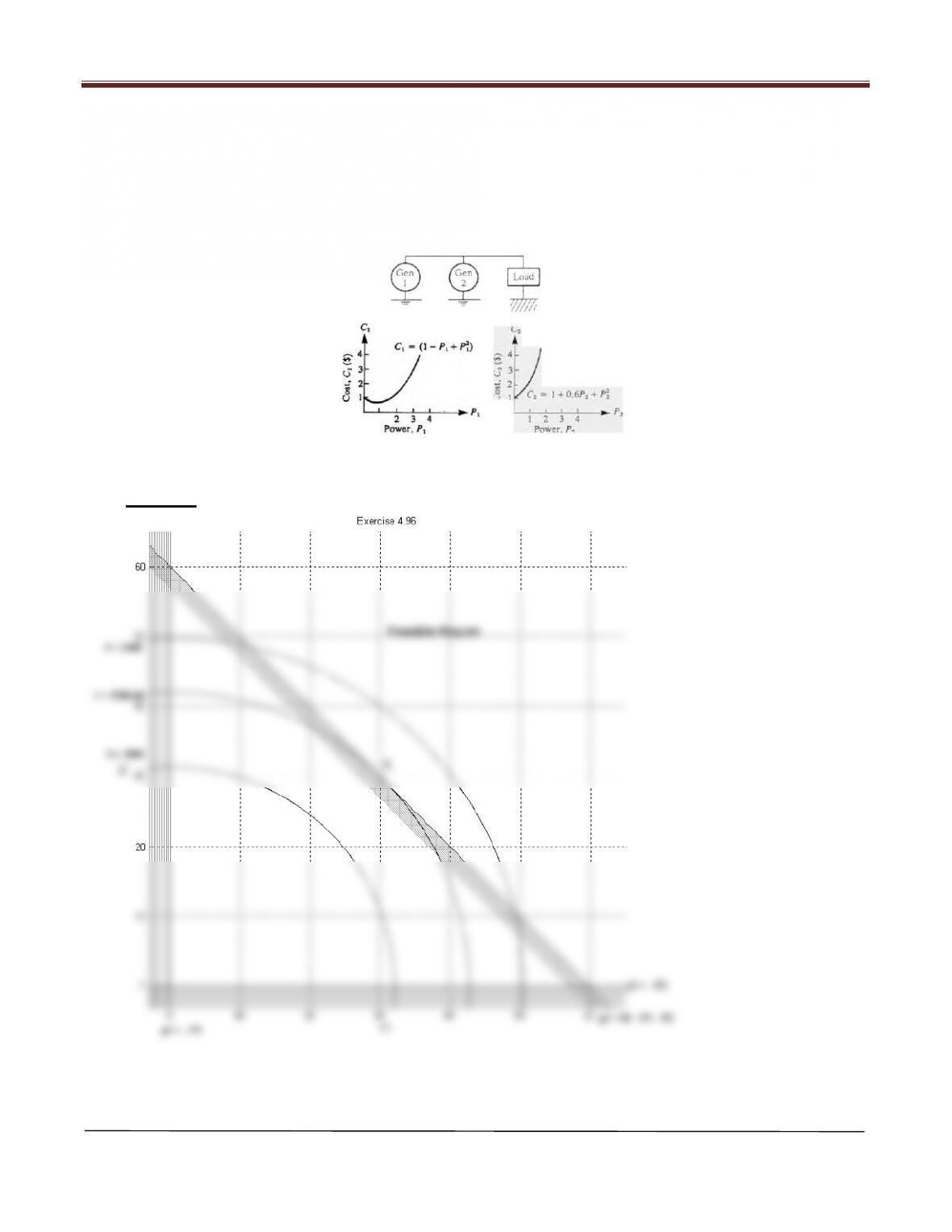
Design the steel framework shown in Fig. E2.13 at a minimum cost. The cost of a horizontal
member in one direction is $20w and in the other direction it is $30d. The cost of a vertical column
is $50h. The frame must enclose a total volume of at least 600 m3. Formulate the design optimization
problem.
FIGURE E2.13 Steel frame.
Solution
Referring to the formulation in Exercise 2.13, we have
Chapter 4 Optimum Design Concepts: Optimality Conditions
Arora, Introduction to Optimum Design, 4e
4-82
4.96________________________________________________________________________________
Two electric generators are interconnected to provide total power to meet the load. Each generator’s
cost is a function of the power output, as shown in Fig. E2.14. All costs and power are expressed on
a per unit basis. The total power needed is at least 60 units. Formulate a minimum cost design
problem to determine the power outputs P1 and P2.
FIGURE E2.14 Power generator.
Solution
Chapter 4 Optimum Design Concepts: Optimality Conditions
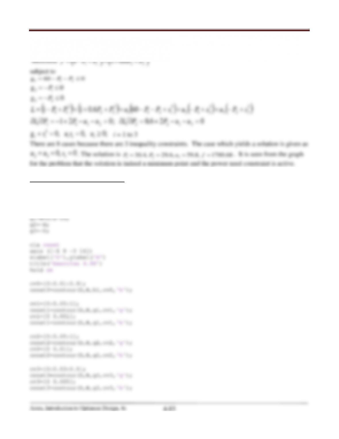
According to the graphical solution, the point A (30, 29) is minimum point.
Referring to the formulation in Exercise 2.14, we have
22
Chapter 4 Optimum Design Concepts: Optimality Conditions
fv=[45000 62512.75 80000];
fs=contour(D,H,f,fv,‘b’);
b=[5.758826];
plot(a,b,‘.k’);
Chapter 4 Optimum Design Concepts: Optimality Conditions
Arora, Introduction to Optimum Design, 4e
4-85
4.97________________________________________________________________________________
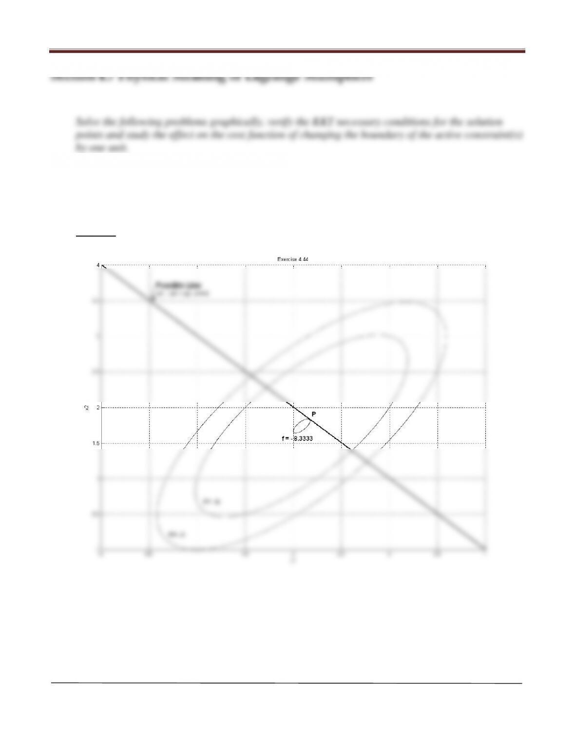
Exercise 4.43
Minimize (1,2)= 41
2+ 32
2−512−81
subject to 1+2−4 = 0
Solution
Chapter 4 Optimum Design Concepts: Optimality Conditions
Referring to Exercise 4.43, the point satisfying the KKT necessary conditions is
The gradient of cost and constraint functions are
These vectors are along the same line.
MATLAB Code for Exercise 4.97
clear all
axis equal
[x1,x2]=meshgrid(–5:0.005:5, –5:0.005:5);
b=[1.83333 1.39237];
plot(a,b,‘.k’)
Chapter 4 Optimum Design Concepts: Optimality Conditions
4.98________________________________________________________________________________
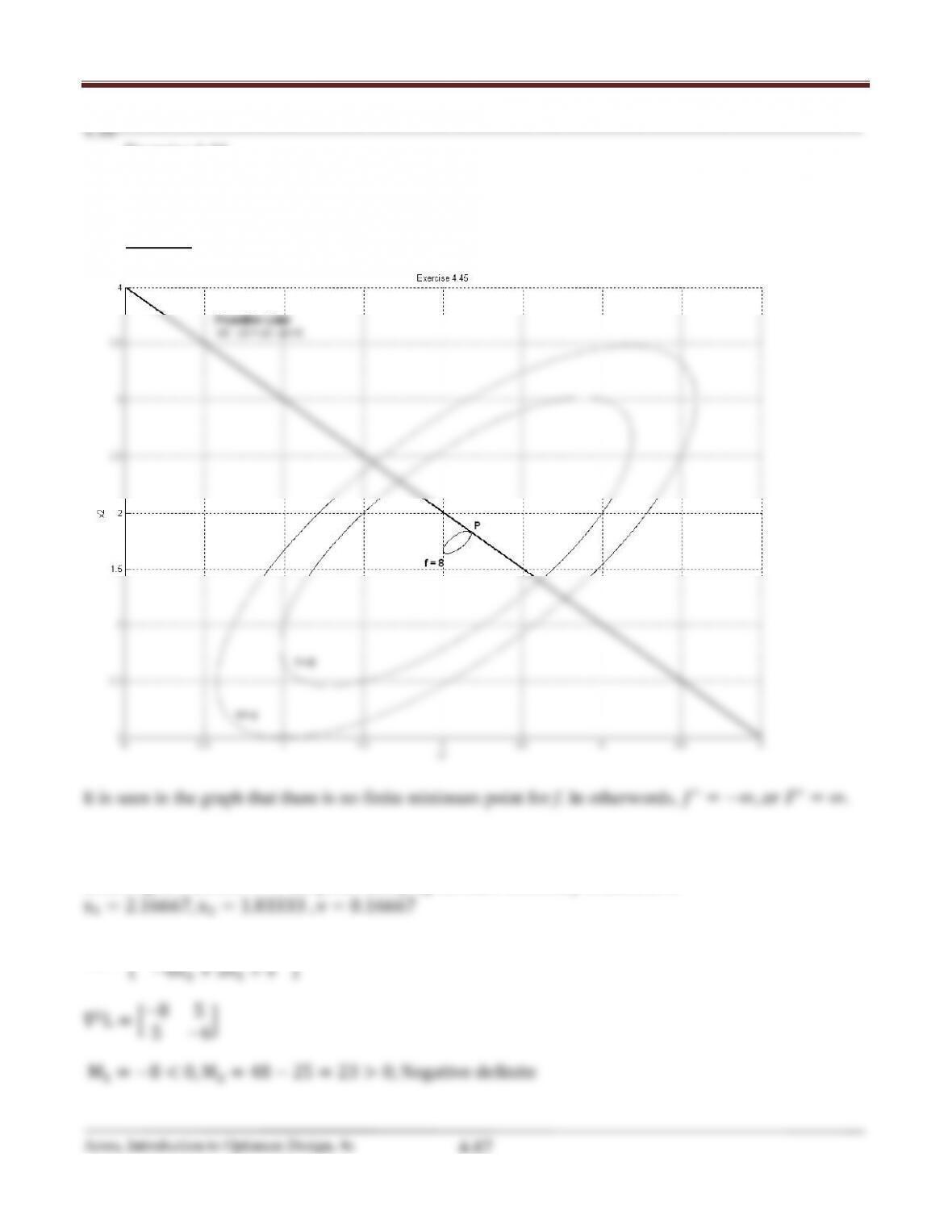
Exercise 4.44
Maximize (1,2)= 41
2+ 32
2−512−81
subject to 1+2−4 = 0
Solution
SECOND ORDER CONDITIONS ARE DISCUSSED IN CHAPTER 5
Referring to Exercise 4.44, the point satisfying the KKT necessary conditions is
∇L = �−8x1+ 5x2+8+ν
Chapter 4 Optimum Design Concepts: Optimality Conditions
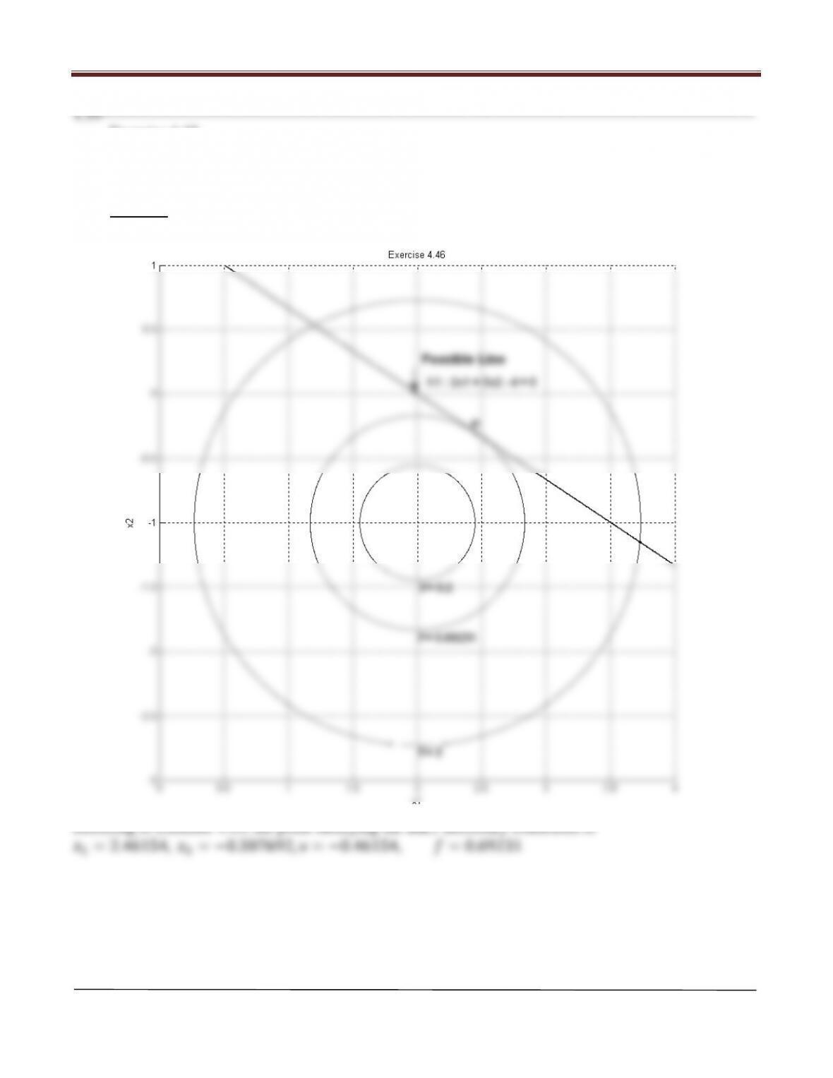
The Hessian of cost function is negative definite. So, this is not a convex problem. This also violates the
second order necessary condition for a local minimum point.
MATLAB Code for Exercise 4.98
clear all
axis equal
[x1,x2]=meshgrid(–5:0.005:5, –5:0.005:5);
fv=[8.3333 6 4];
fs=contour(x1,x2,f,fv,‘b’);
b=[1.83333];
plot(a,b,‘.k’)
Chapter 4 Optimum Design Concepts: Optimality Conditions
Arora, Introduction to Optimum Design, 4e
4-89
Exercise 4.45
Minimize (1,2)= (1−2)2+ (2+ 1)2
subject to 21+ 32−4 = 0
Solution
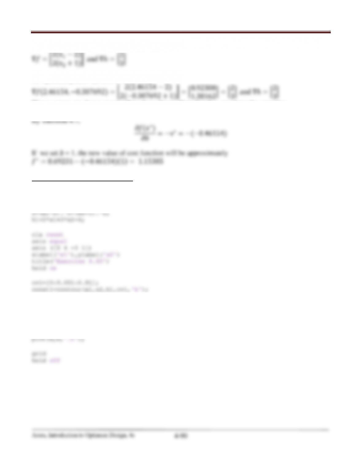
Referring to Exercise 4.45, the point satisfying the KKT necessary conditions is
SECOND ORDER CONDITIONS ARE DISCUSSED IN CHAPTER 5
The Hessian of cost function is positive definite, and the constraint function is linear. So, this is a
convex problem. It follows from Theorem 4.11 that the point is an isolated global minimum.
Chapter 4 Optimum Design Concepts: Optimality Conditions
The gradient of cost and constraint functions are
At optimum point P (2.46154, -0.307692)
These vectors are shown at point P in above figure. Note that they are along the same line.
MATLAB Code for Exercise 4.99
clear all
axis equal
[x1,x2]=meshgrid(0:0.005:4, –3:0.005:1);
fv=[0.2 0.69231 3];
fs=contour(x1,x2,f,fv,‘b’);
a=[2.46154 3.72551];
b=[–0.307692 –1.15034];