Chapter 4 Optimum Design Concepts
MATLAB Code for Exercise 122
clear all
axis equal
[x1,x2]=meshgrid(–2:0.01:8, –2:0.01:8);
f=(x1–3).^2+(x2–3).^2;
b=[0.75];
plot(a,b,‘.k’);
Chapter 4 Optimum Design Concepts
Arora, Introduction to Optimum Design, 4e
4-158
4.123_______________________________________________________________________________
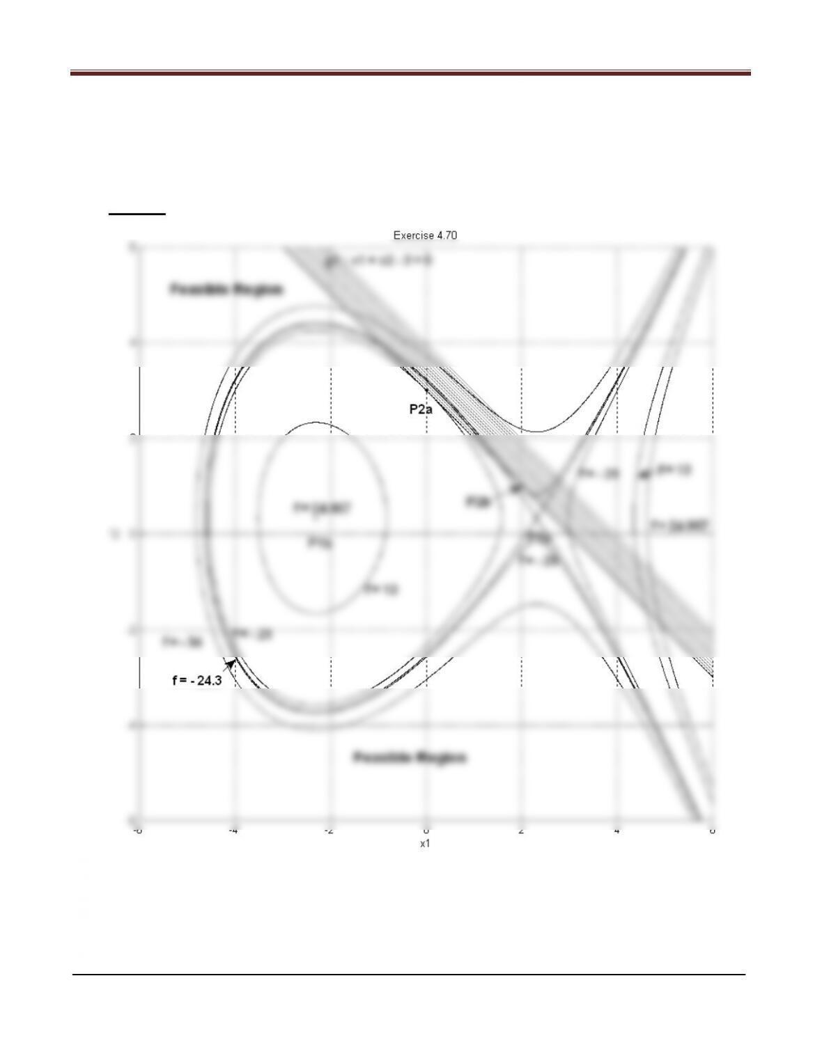
Exercise 4.70
Minimize (1,2)=1
3−161+ 22−32
2
subject to 1+2≤3
Solution
Chapter 4 Optimum Design Concepts
We need to find isolated or local minimum point(s) which satisfy both KKT necessary conditions and
sufficient or the second order necessary conditions.
Referring to Exercise 4.70, the points satisfying the KKT necessary conditions are
x1
∗
x2
∗
u1
∗
P1a
4
√3
1
3
0
P1b
−4
√3
1
3
0
P2a
0
3
16
P2b
2
1
4
SECOND ORDER CONDITIONS ARE DISCUSSED IN CHAPTER 5
1. At point P1a �4
√3,1
3�,
Since no constraint is active, Hessian of Lagrangian must be positive definite throughout to satisfy
2. At point P2a(0, 3),
∇2L = �0 0
0−6�
Chapter 4 Optimum Design Concepts
Arora, Introduction to Optimum Design, 4e
4-160
MATLAB Code for Exercise 123
clear all
axis equal
[x1,x2]=meshgrid(–6:0.01:6, –6:0.01:6);
cv1=[0:0.07:1];
const1=contour(x1,x2,g1,cv1,‘g’);
cv1=[0 0.001];
const1=contour(x1,x2,g1,cv1,‘k’);
Chapter 4 Optimum Design Concepts
Arora, Introduction to Optimum Design, 4e
4-161
4.124_______________________________________________________________________________
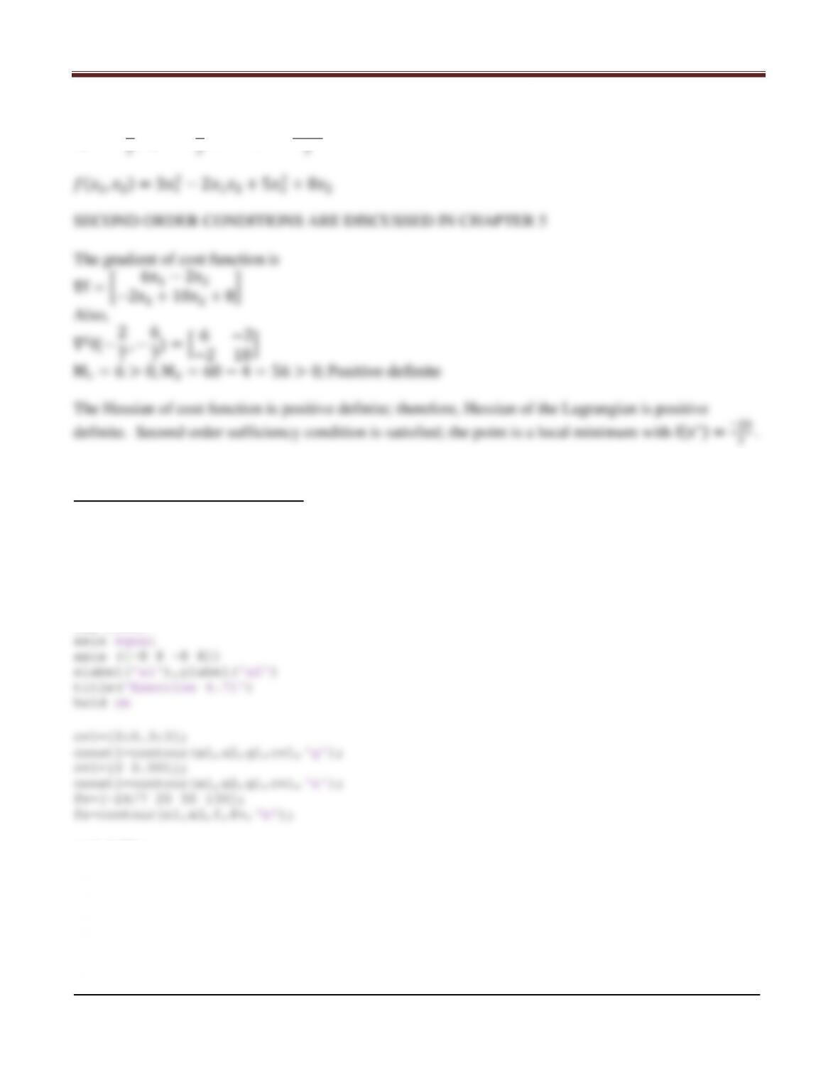
Exercise 4.71
Minimize (1,2)= 31
2−212+ 52
2+ 82
subject to 1
2−2
2+ 82≤16
Solution
Chapter 4 Optimum Design Concepts
Arora, Introduction to Optimum Design, 4e
4-162
Referring to Exercise 4.71, the point satisfying the KKT necessary conditions is
x1=−2
MATLAB Code for Exercise 124
clear all
axis equal
[x1,x2]=meshgrid(–8:0.01:8, –8:0.01:8);
f=3*x1.^2–2*x1.*x2+5*x2.^2+8*x2;
g1=x1.^2–x2.^2+8*x2–16;
cla reset
a=[–2/7];
b=[–6/7];
plot(a,b,‘.k’);
grid
hold off
Chapter 4 Optimum Design Concepts
Arora, Introduction to Optimum Design, 4e
4-163
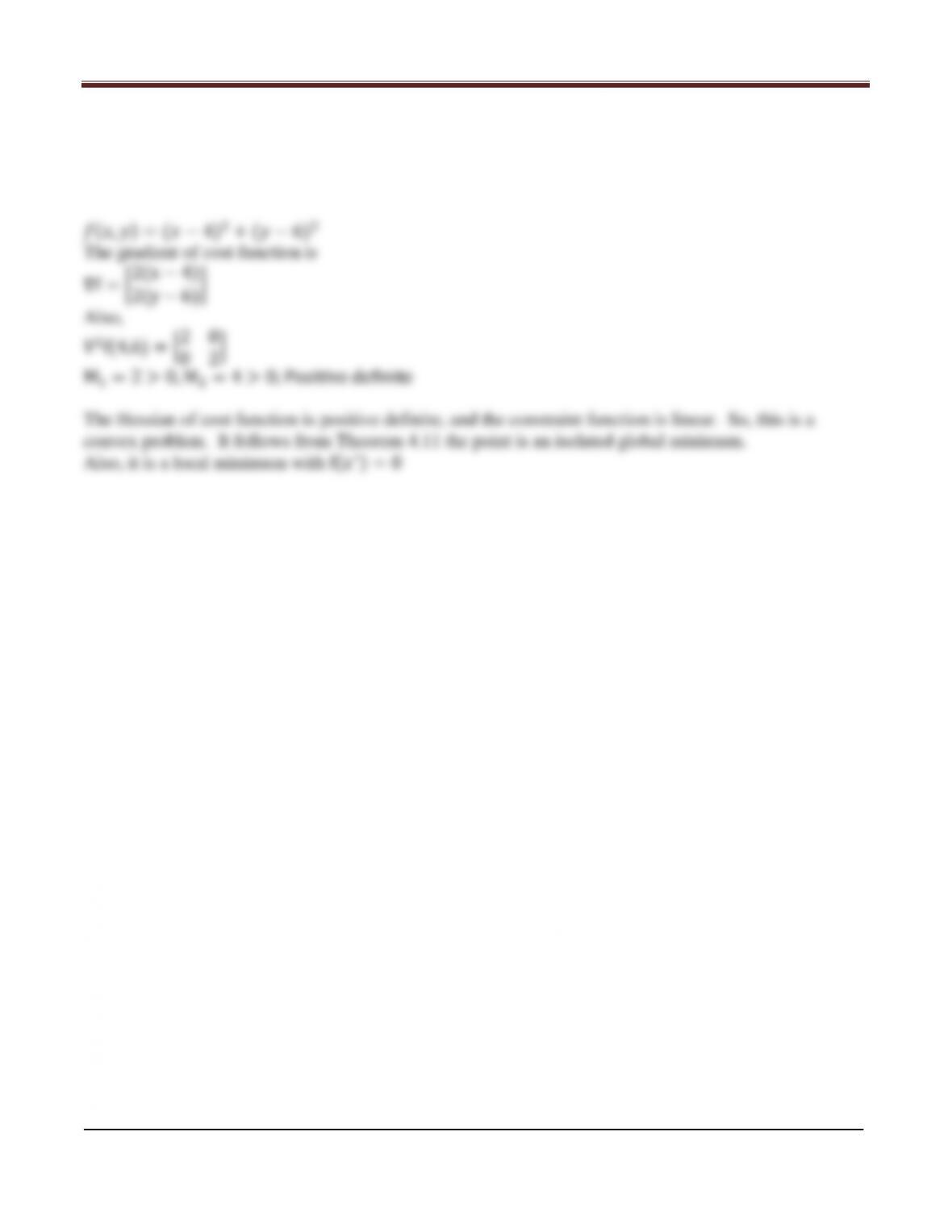
Exercise 4.72
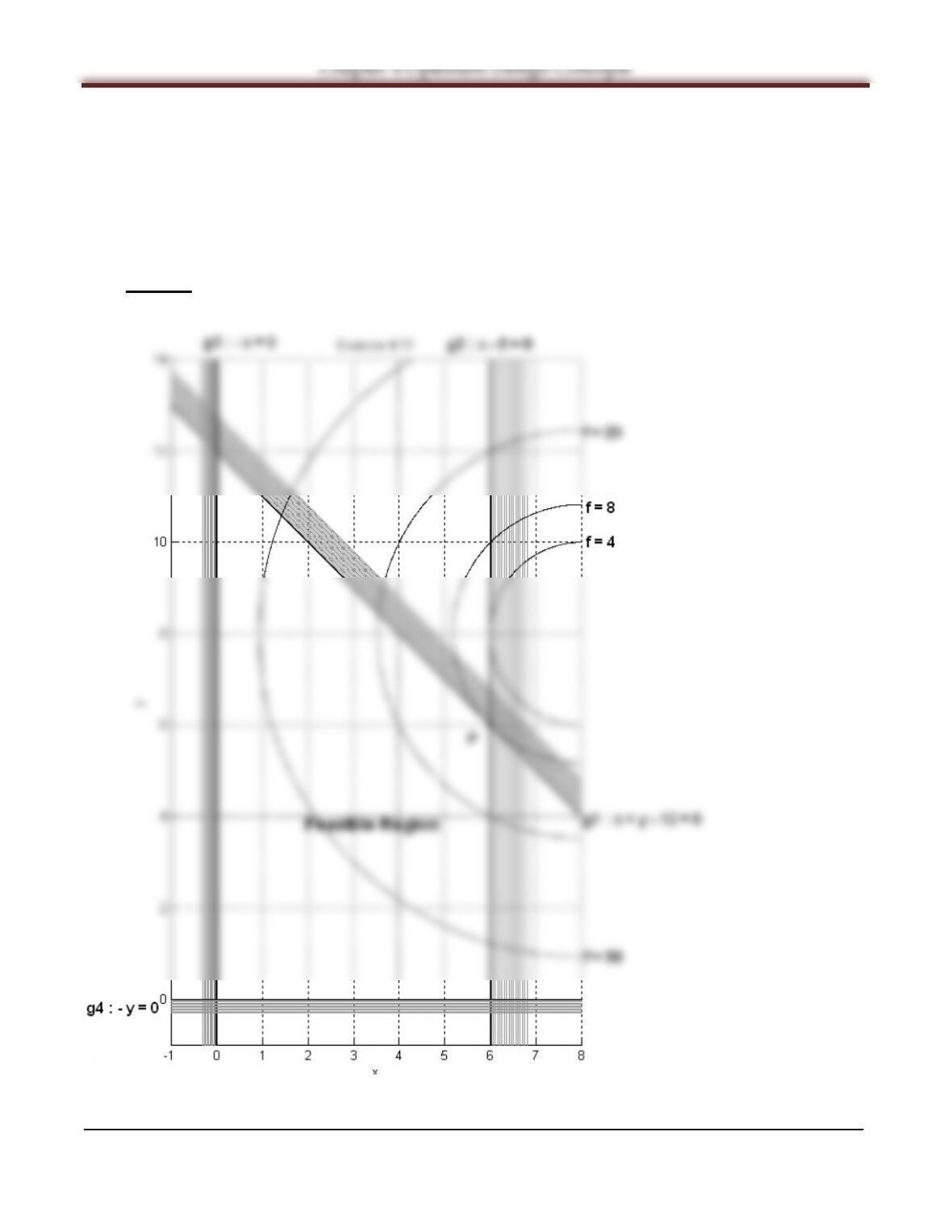
Minimize (,)= (−4)2+ ( −6)2
subject to + ≤ 12
≤ 6
, ≥ 0
Solution
Chapter 4 Optimum Design Concepts
Arora, Introduction to Optimum Design, 4e
4-164
Referring to Exercise 4.72, the point satisfying the KKT necessary conditions is
x = 4, y = 6 , u = 0, f = 0
SECOND ORDER CONDITIONS ARE DISCUSSED IN CHAPTER 5
Chapter 4 Optimum Design Concepts
MATLAB Code for Exercise 125
clear all
axis equal
[x,y]=meshgrid(–1:0.01:8, 2:0.01:10);
f=(x–4).^2+(y–6).^2;
cv1=[0:0.05:0.8];
const1=contour(x,y,g1,cv1,‘g’);
cv1=[0 0.01];
const1=contour(x,y,g1,cv1,‘k’);
cv2=[0:0.05:0.8];
const4=contour(x,y,g4,cv4,‘k’);
fv=[0 1 4 9];
fs=contour(x,y,f,fv,‘b’);
a=[4];
b=[6];
Arora, Introduction to Optimum Design, 4e
4-166
4.126_______________________________________________________________________________
Exercise 4.73
Minimize (,)= (−8)2+ ( −8)2
subject to + ≤ 12
≤ 6
, ≥ 0
Solution
Chapter 4 Optimum Design Concepts
Referring to Exercise 4.73, the points satisfying the KKT necessary conditions are
x = y = 6, u1= 4, u2= 0, u3= 0, u4= 0 and f = 8
SECOND ORDER CONDITIONS ARE DISCUSSED IN CHAPTER 5
The Hessian of cost function is positive definite, and the constraint function is linear. So, this is a
convex problem. It follows from Theorem 4.11 the point is an isolated global minimum.
(,)= ( −8)2+ ( −8)2
At optimum point P (6, 6)
∇f(6, 6)=�2(6−8)
2(6−8)�=�−4
−4�
We need to check (4.52) from P.131
− ∇f = u1∇g1+ u2∇g2+ u3∇g3+ u4∇g4
∂f(x∗)
∂e3=−u3∗=−(0)
∂f(x∗)
∂e4=−u4∗=−(0)
If we set e1=1, the new value of cost function will be approximately
MATLAB Code for Exercise 126
clear all
axis equal
[x,y]=meshgrid(–1:0.01:8, –1:0.01:14);
f=(x–8).^2+(y–8).^2;
cv1=[0:0.05:0.8];
const1=contour(x,y,g1,cv1,‘g’);
cv1=[0 0.01];
const1=contour(x,y,g1,cv1,‘k’);
cv2=[0:0.05:0.8];
const4=contour(x,y,g4,cv4,‘k’);
fv=[4 8 20 50];
fs=contour(x,y,f,fv,‘b’);
a=[6];
b=[6];
Chapter 4 Optimum Design Concepts
Arora, Introduction to Optimum Design, 4e
4-169
4.127_______________________________________________________________________________
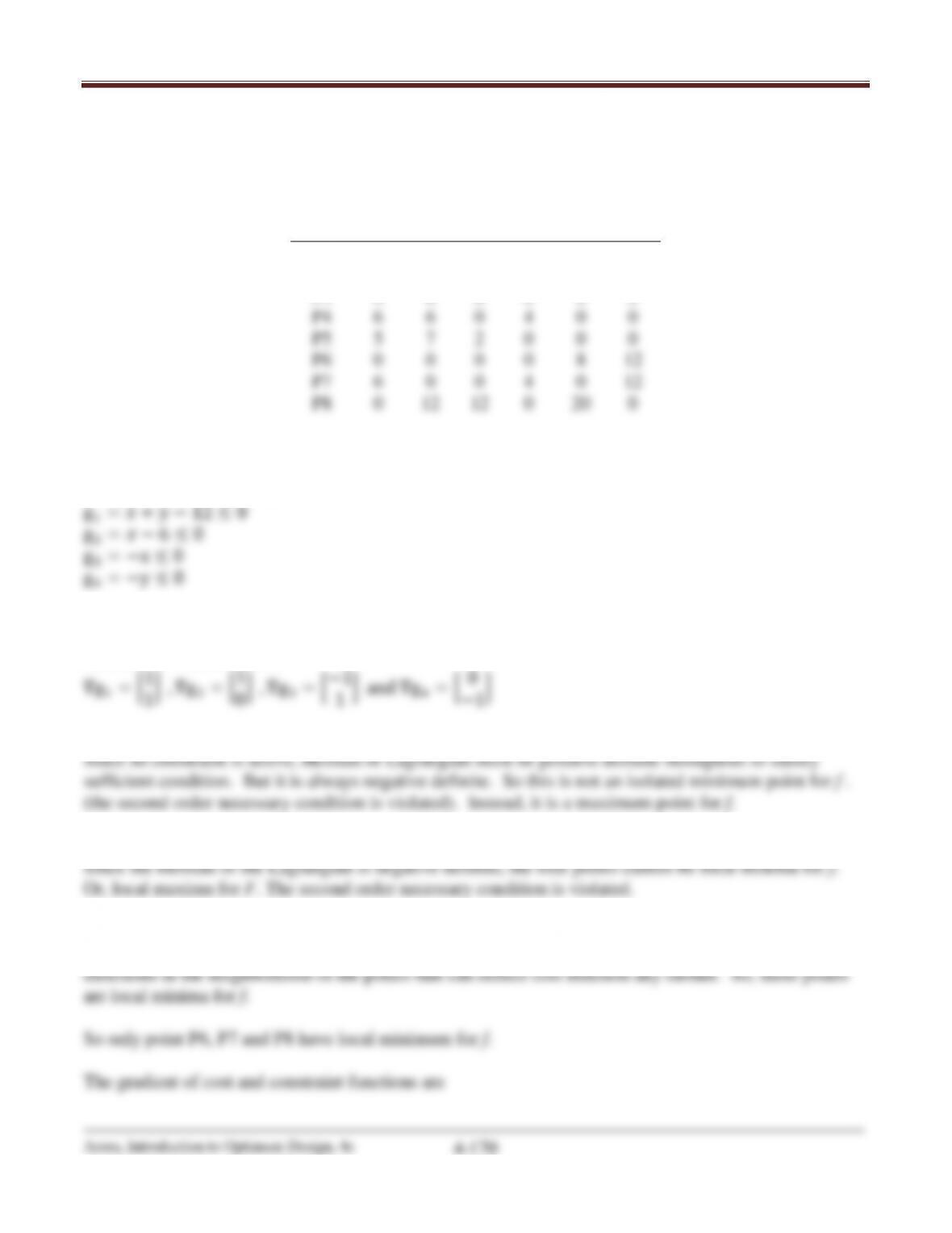
Exercise 4.74
Maximize (,)= ( −4)2+ (−6)2
subject to + ≤ 12
6≥
, ≥ 0
Solution
Chapter 4 Optimum Design Concepts
We need to find isolated or local minimum point(s) which satisfy both KKT necessary conditions and
sufficient or the second order necessary conditions.
Referring to Exercise 4.74, the points satisfying the KKT necessary conditions are
x
y
u1
u2
u3
u4
P1
4
6
0
0
0
0
P2
4
0
0
0
0
12
P3
0
6
0
0
8
0
P4
6
6
0
4
0
0
P5
5
7
2
0
0
0
P6
0
0
0
0
8
12
P7
6
0
0
4
0
12
P8
0
12
12
0
20
0
SECOND ORDER CONDITIONS ARE DISCUSSED IN CHAPTER 5
(,)=−(−4)2−(−6)2
∇2L = �−2 0
0−2�; M1=−2 < 0, M2= 4 > 0; Negative definite
Gradient of constraints are
1. At point P1 (4, 6)
2. At points P2 (4, 0), P3 (0,6) , P4 (6,6)and P5 (5,7)
3. At points P6 (0, 0) and P7 (6, 0)
The number of active constraints is equal to the number of design variables. There are no feasible
Chapter 4 Optimum Design Concepts
Arora, Introduction to Optimum Design, 4e
4-171
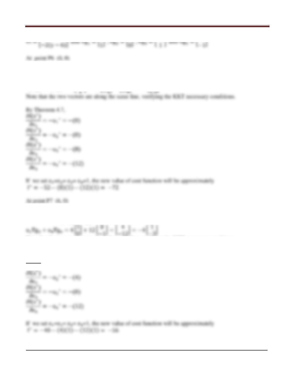
By (4.52),
−∇f(0, 0)=−�−2(0 −4)
−2(0 −6)�=−8�1
1.5� and
u3∇g3+ u4∇g4= 8 �−1
By (4.52),
−∇f(6, 0)=−�−2(6 −4)
−2(0 −6)�=−4�1
−3� and
Note that the two vectors are along the same line, verifying the KKT necessary conditions.
By Theorem 4.7,
∂f(x∗)
∂e1=−u1∗=−(0)
Chapter 4 Optimum Design Concepts
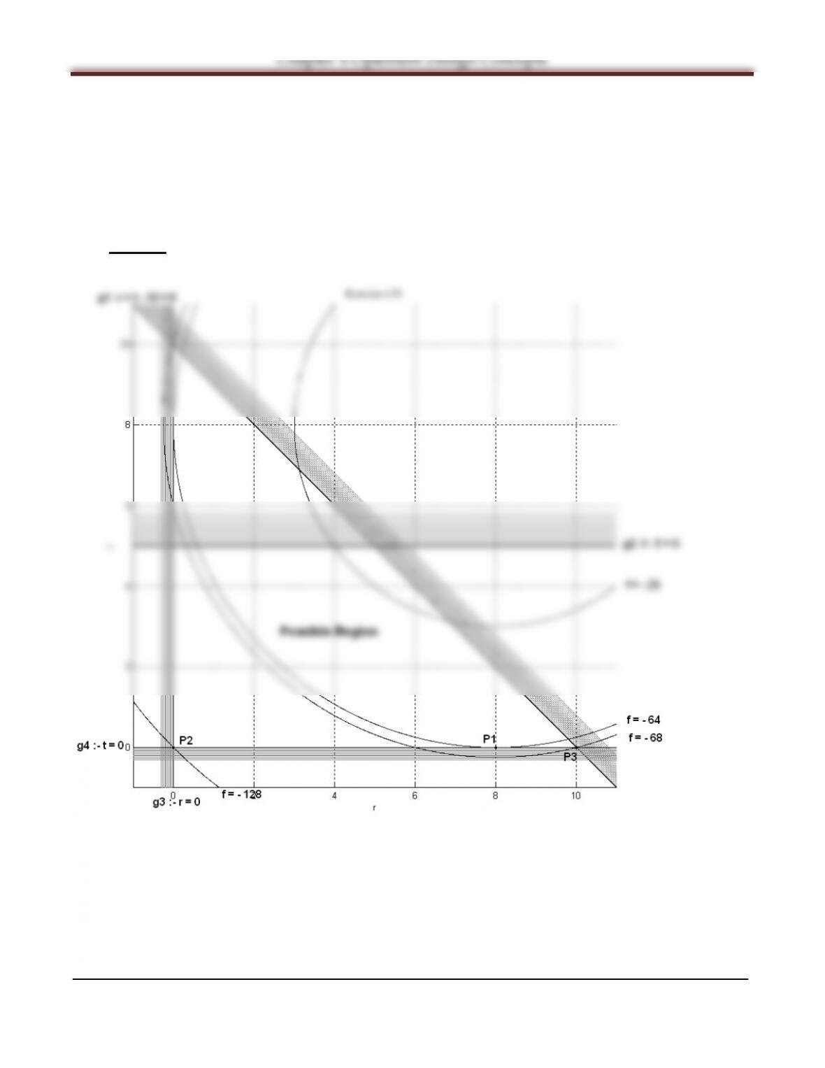
MATLAB Code for Exercise 127
clear all
axis equal
[x,y]=meshgrid(–4:0.01:12, –2:0.01:14);
f=(–1)*((x–4).^2+(y–6).^2);
cv1=[0:0.05:0.8];
const1=contour(x,y,g1,cv1,‘g’);
cv1=[0 0.01];
const1=contour(x,y,g1,cv1,‘k’);
cv2=[0:0.05:0.8];
const4=contour(x,y,g4,cv4,‘k’);
fv=[–52 –40 –36 –16 –4 –2 0];
fs=contour(x,y,f,fv,‘b’);
a=[4 6 0 6 5 0 6 0 6 4];
b=[6 0 6 6 7 0 0 12 6 0];
Arora, Introduction to Optimum Design, 4e
4-173
4.128_______________________________________________________________________________
Exercise 4.75
Maximize (,)= (−8)2+ ( −8)2
subject to 10 ≥ +
≤ 5
, ≥ 0
Solution
Chapter 4 Optimum Design Concepts
We need to find isolated or local minimum point(s) which satisfy both KKT necessary conditions and
sufficient or the second order necessary conditions.
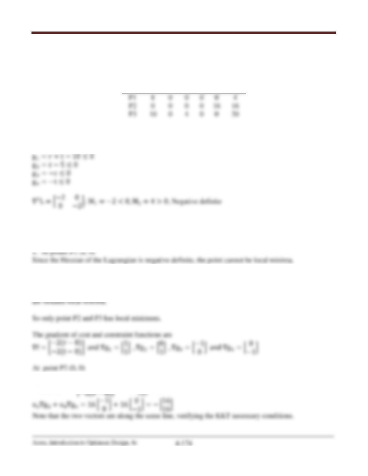
Referring to Exercise 4.75, the points satisfying the KKT necessary conditions are
r
t
u1
u2
u3
u4
P1
8
0
0
0
0
4
P2
0
0
0
0
16
16
P3
10
0
4
0
0
20
SECOND ORDER CONDITIONS ARE DISCUSSED IN CHAPTER 5
(,)=−(−8)2−(−8)2
Gradient of constraints are
∇g1=�1
1� , ∇g2=�0
1� , ∇g3=�−1
0� and ∇g4=�0
−1�
2. At point P2 (0,0) and P3 (10, 0)
The number of active constraints is equal to the number of design variables. There are no feasible
directions in the neighborhood of the points that can reduce cost function any further. So, these points
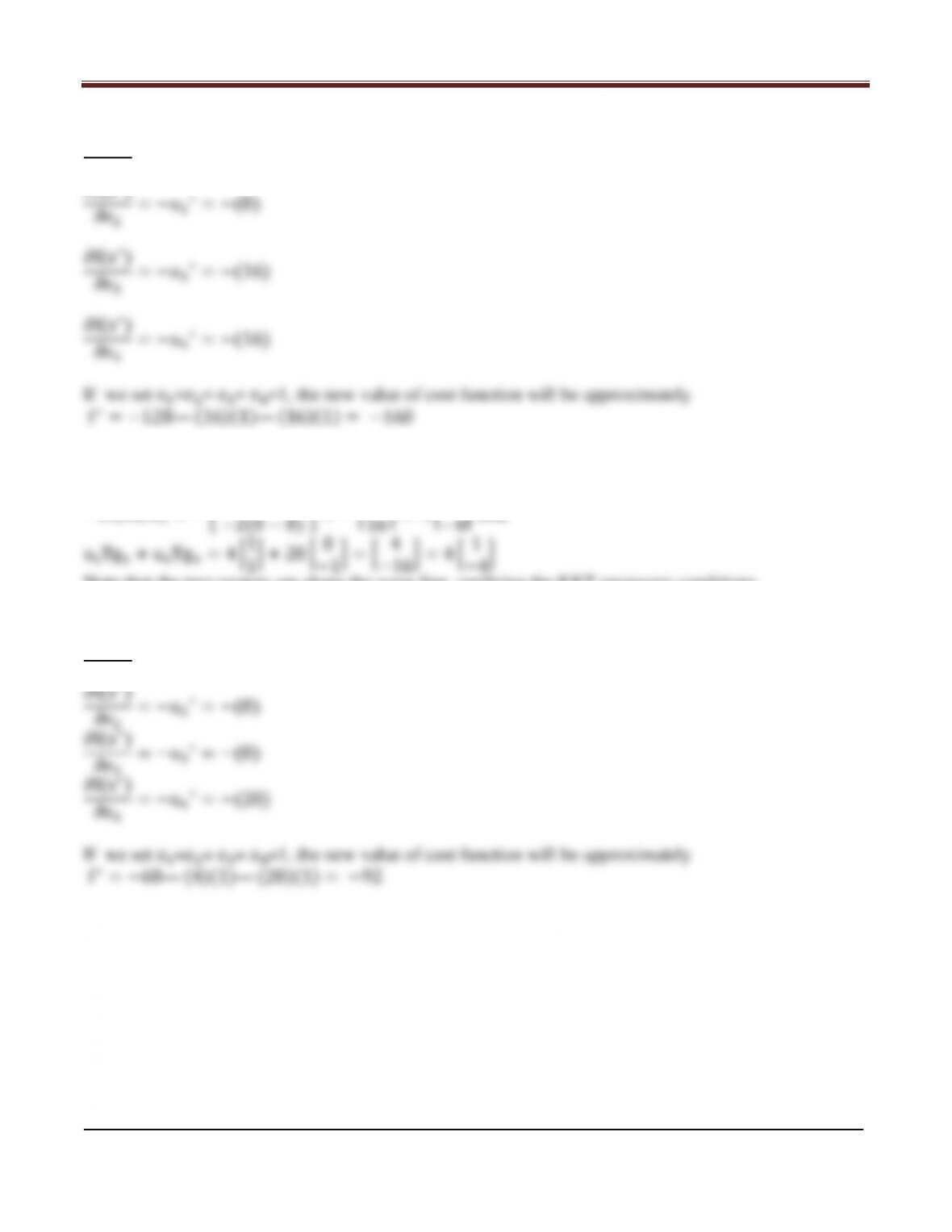
By (4.52),
−∇f(0, 0)=−�−2(0 −8)
Chapter 4 Optimum Design Concepts
Arora, Introduction to Optimum Design, 4e
4-175
By Theorem 4.7,
∂f(x∗)
∂e1=−u1∗=−(0)
∂f(x∗)
At point P3 (10, 0)
By (4.52),
−∇f(10, 0)=−�−2(10 −8)
Note that the two vectors are along the same line, verifying the KKT necessary conditions.
By Theorem 4.7,
∂f(x∗)
∂e1=−u1∗=−(4)
Chapter 4 Optimum Design Concepts
MATLAB Code for Exercise 128
clear all
axis equal
[r,t]=meshgrid(–1:0.01:11, –1:0.01:11);
f=(–1)*((r–8).^2+(t–8).^2);
cv1=[0:0.05:0.8];
const1=contour(r,t,g1,cv1,‘g’);
cv1=[0 0.01];
const1=contour(r,t,g1,cv1,‘k’);
cv2=[0:0.05:0.8];
const4=contour(r,t,g4,cv4,‘k’);
fv=[–25 –64 –68 –128];
fs=contour(r,t,f,fv,‘b’);
a=[8 0 10];
b=[0 0 0];