Chapter 4 Optimum Design Concepts: Optimality Conditions
4.73____________________________________________________________________________
Minimize (,)= ( − 8)2+ ( − 8)2
subject to + ≤ 12
≤ 6
, ≥ 0
Solution
Minimize
( ) ( ) ( )
22
1
, 8 8 ; subject to g 12 0;f xy x y x y= − + − =+− ≤
i = 1 to 4 (there are 16 cases).
Case 2.
123 4
0, 0;uuu s= = = =
gives no candidate point.
124 3
Case 4.
134 2
0, 0;uuu s= = = =
gives no candidate point.
8=
Case 6.
;0 ,0
4321
==== ssuu
gives no candidate point.
;0 ,0
4231
Case 8.
;0 ,0
3241
==== ssuu
gives no candidate point.
;0 ,0
4132
Case 10.
2 4 13
0, 0;uu ss= = = =
gives no candidate point.
Case 11.
;0 ,0
2143
==== ssuu
gives
( )
6, 6
as a KKT point with u1 = 4; f
8=
.
Case 13.
;0 ,0
4312
==== sssu
gives no candidate point.
Case 16.
0
==== ssss
; gives no candidate point.
case 11,
( )
g 1, 1=Ñ
,
( )
g 1,0=Ñ
. Since
gÑ
and
gÑ
are linearly independent regularity is
4.74________________________________________________________________________________
Maximize (,)= ( − 4)2+ ( − 6)2
subject to + ≤ 12
6≥
, ≥ 0
Solution
Minimize
( ) ( ) ( )
22
1
, 4 6 ; subject to g 12 0;f xy x y x y=− − − − =+− ≤
g 6 0; g 0; g 0;x xy=−≤ =−≤ =−≤
2
4
0;
ys
−+ =
;0 ;0 ≥=
iii
usu
i = 1 to 4 (there are 16 cases).
Case 1.
1234
0;uuuu= = = =
gives
( )
4, 6
as a KKT point ; F
0=
.
( )
5, 7
2=
Case 3.
134 2
0, 0;uuu s= = = =
gives
( )
6, 6
as a KKT point with u2 = 4; F
4=
. Note that for this
Case 4.
124 3
0, 0;uuu s= = = =
gives
( )
0, 6
as a KKT point with u3 =8; F
16=
.
123 4
0, 0;uuu s= = = =
4, 0
Case 6.
;0 ,0
==== ssuu
gives
( )
6, 6
as a KKT point with u1 = 0, u2 = 4; F
4=
. Note that
Case 7.
;0 ,0
3241
==== ssuu
gives no candidate point.
;0 ,0
4321
( )
0, 0
Case 9.
;0 ,0
4132
==== ssuu
gives no candidate point.
;0 ,0
==== ssuu
6, 0

Chapter 4 Optimum Design Concepts: Optimality Conditions
;0 ,0
Case 13.
;0 ,0
==== sssu
gives no candidate point.
Case 16.
0
4321
==== ssss
; gives no candidate point.
Check for regularity: For cases 1, 2, 3, 4 and 5, there is only one active constraint, so regularity is
satisfied. For case 6,
( ) ( )
g 1, 0 , g 0, 1∇=− ∇= −
. Since
g∇
and
g∇
are linearly independent,
g∇
g∇
g∇
g∇
Chapter 4 Optimum Design Concepts: Optimality Conditions
4.75________________________________________________________________________________
Maximize (,)= ( − 8)2+ ( − 8)2
subject to 10 ≥ +
≤ 5
, ≥ 0
Solution
Minimize
( ) ( ) ( )
22
, 8 8 ; subject to g 10 0;f rt r t r t=− − − − = +− ≤
;0 ;0 ≥=
iii
usu
i = 1 to 4 (there are 16 cases).
Case 2.
0, 0;uuu s= = = =
gives
( )
8, 0
as a KKT point with u4 = 16; F
64=
.
124 3
0, 0;uuu s= = = =
Case 5.
234 1
0, 0;uuu s= = = =
gives no candidate point.
;0 ,0
4321
Case 7.
;0 ,0
4231
==== ssuu
gives no candidate point.
;0 ,0
3241
;0 ,0
4132
Case 10.
0, 0;uu ss= = = =
gives no candidate point.
;0 ,0
2143
;0 ,0
Case 13.
;0 ,0
==== sssu
gives no candidate point.
Case 16.
0
==== ssss
; gives no candidate point.

Chapter 4 Optimum Design Concepts: Optimality Conditions
Arora, Introduction to Optimum Design, 4e
4-45
Check for regularity: For cases 2, there is only one active constraint, so regularity is satisfied. For
Chapter 4 Optimum Design Concepts: Optimality Conditions
4.76________________________________________________________________________________
Maximize (,)= ( − 3)2+ ( − 2)2
subject to 10 ≥ +
≤ 5
, ≥ 0
Solution
Minimize
( ) ( ) ( )
22
, 32
f rt r t
=−− −−
i = 1 to 4 (there are 16 cases).
Case 1.
1234
0;uuuu= = = =
Case 2.
0, 0;uuu s= = = =
Case 3.
0, 0;uuu s= = = =
Case 4.
0, 0;uuu s= = = =
Case 5.
0, 0;uuu s= = = =
Case 6.
;0 ,0
==== ssuu
;0 ,0
Case 8.
;0 ,0
==== ssuu

Case 9.
;0 ,0
==== ssuu
Case 10.
2 4 13
0, 0;uu ss= = = =
;0 ,0
Case 12.
0 ,0 3214 ==== sssu
; gives no candidate point.
4321
Check for regularity: For cases 1, 2, 3, 4 and 5, there is only one active constraint, so regularity is
satisfied. For case 6,
( ) ( )
g 1, 0 , g 0, 1∇=− ∇= −
. Since
g∇
and
g∇
are linearly independent,
g∇
g∇
g∇
g∇
Chapter 4 Optimum Design Concepts: Optimality Conditions
4.77________________________________________________________________________________
Maximize (,)= ( − 8)2+ ( − 8)2
subject to + ≤ 10
≥ 0
≤ 0
Solution
Minimize
( ) ( ) ( )
22
1
, 8 8 ; subject to g 10 0;f rt r t r t=− − − − = +− ≤
i = 1 to 3 (there are 8 cases).
Case 1.
0uuu= = =
; no candidate minimum.
Case 3.
13 2
0, 0uu s= = =
; no candidate minimum.
Case 4.
0, 0uu s= = =
; no candidate minimum.
Case 6.
2 13
0, 0u ss= = =
; no candidate minimum.
Case 8.
0sss= = =
; no candidate minimum.
Chapter 4 Optimum Design Concepts: Optimality Conditions
4.78________________________________________________________________________________
Maximize (,)= ( − 3)2+ ( − 2)2
subject to 10 ≥ +
≥ 5
, ≥ 0
Solution
Minimize
( ) ( )
( )
22
1
, 3 2 ; subject to g 10 0;f rt r t r t=− − − − = +− ≤
;0 ;0 ≥=
iii
usu
i = 1 to 4 (there are 16 cases).
Case 2.
123 4
0, 0;uuu s= = = =
gives no candidate point.
124 3
Case 4.
0, 0;uuu s= = = =
gives
3, 5
as a KKT point with u3 = 6; F =9.
234 1
;0 ,0
4321
Case 7.
;0 ,0
4231
==== ssuu
gives no candidate point.
;0 ,0
3241
Case 9.
;0 ,0
4132
==== ssuu
gives no candidate point.
Case 11.
;0 ,0
2143
==== ssuu
gives no candidate point.
;0 ,0
4321
Case 13.
;0 ,0
4312
==== sssu
gives no candidate point.
0 ,0 4213 ==== sssu
Case 15.
0 ,0 3214 ==== sssu
; gives no candidate point.
Case 16.
0
==== ssss
; gives no candidate point.
case 10,
( )
g 1, 1=Ñ
,
( )
g 1, 0= −Ñ
. Since
gÑ
and
gÑ
are linearly independent regularity is
Chapter 4 Optimum Design Concepts: Optimality Conditions
4.79________________________________________________________________________________
Consider the problem of designing the “can” formulated in Section 2.2. Write KKT conditions and
solve them. Interpret the necessary conditions at the solution point graphically.
Solution
Minimize
( )
2 ,
2
DDHHDf π+π=
,
subject to
2
1
g 400 4 0;DH= −π ≤
;04 ;02 541
2
321 =+−π−π=∂∂=+−π−π+π=∂∂ uuuDDHLuuDHuDHDL
2
g 0, 0, 0; 1 to 5.
s us u i+= = ≥ =
4.80________________________________________________________________________________
A minimum weight tubular column design problem is formulated in Section 2.7 using mean radius
R and thickness t as design variables. Solve the KKT conditions for the problem imposing an
additional constraint R/t ≤ 50 for the following data: P = 50kN, l = 5.0m, E = 210GPa,=250MPa
and =7850kg/m3. Interpret the necessary conditions at the solution point graphically.
Solution
Use kilograms, Newtons and meters as units: P = 50 kN = 5
4
10×
N, l = 5.0 m, E = 210 GPa =
( ) ( )( )( )
kg ,0261524605785022 tRRtRtltRf .,., =π=πρ=
8
g 2 7 957 75 2 5 10 0
P Rt Rt= π− = − × ≤.. .s
2
2
1
1
( ) ( ) ( )
2
55
2
44
2
33 50 stusRustRu +−++−++−+
21123
At this point
145
g , g , g
are < 0. All the KKT conditions are satisfied, so
Chapter 4 Optimum Design Concepts: Optimality Conditions
4.81________________________________________________________________________________
A minimum weight tubular column design problem is formulated in Section 2.7 using outer radius
Ro and inner radius Ri as design variables. Solve the KKT conditions for the problem imposing an
additional constraint 0.5(Ro+ Ri)/(Ro−Ri)≤50. Use the same data as in Exercise 4.80.
Interpret the necessary conditions at the solution point graphically.
Solution
Referring to the Formulation 2 in Section 2.7 and Exercise 4.80, we have
( )
( )
( )( )
( ) ( )( )
22 22 522
, 7850 5 1 2331 10
oi oi oi oi
fRR lRR RR RR=πρ −=π −= × −.
( )
( )( )
( )
2
22
1
5
491591521046622
ioooi
RRuRRRL −−×=∂∂ ..
( )
( )
2
10 3
23 5
4 1.62783 10 0
i ooi
Ru u R R R u+ × + − −=
2
g 0, 0, 0; 1 to 5
i i ii i
s us u i+= = ≥ =
There are 32 cases because there are five inequality constraints. The case which yields a solution
is
.ssuuu 0 ,0
32541
=
====
Solving this case, we get
Arora, Introduction to Optimum Design, 4e
4-53
4.82________________________________________________________________________________
An engineering design problem is formulated as
Minimize (1,2)=1
2+32012
Subject to 1
6021−1≤0
1−1
3600 1(1− 2)≤0
1,2≥0
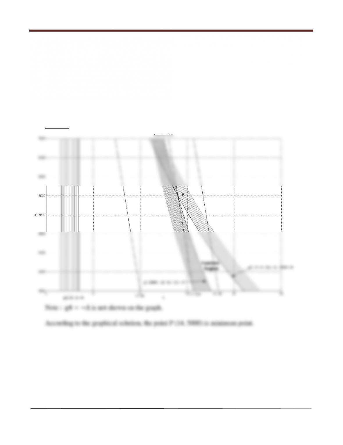
Write KKT necessary condition and solve for the candidate minimum designs. Verify the solutions
graphically. Interpret the KKT conditions on the graph for the problem.
Solution
Minimize
( )
,320 21
2
1xxxf +=x
subject to
11 2
g 60 1 0;xx= −≤
Chapter 4 Optimum Design Concepts: Optimality Conditions
Arora, Introduction to Optimum Design, 4e
4-54
Formulate and solve the following problems graphically. Verify the KKT conditions at the solution point
and show gradients of the cost function and active constraints on the graph.
4.83________________________________________________________________________________
A 100 ×100m lot is available to construct a multistory office building. At least 20,000 m2 total
floor space is needed. According to a zoning ordinance, the maximum height of the building can
be only 21m, and the area for parking outside the building must be at least 25 percent of the floor
area. It has been decided to fix the height of each story at 3.5m. The cost of the building in millions
of dollars is estimated at 0.6 h +0.001 A, where A is the cross-sectional area of the building per
floor and h is the height of the building. Formulate the minimum cost design problem.
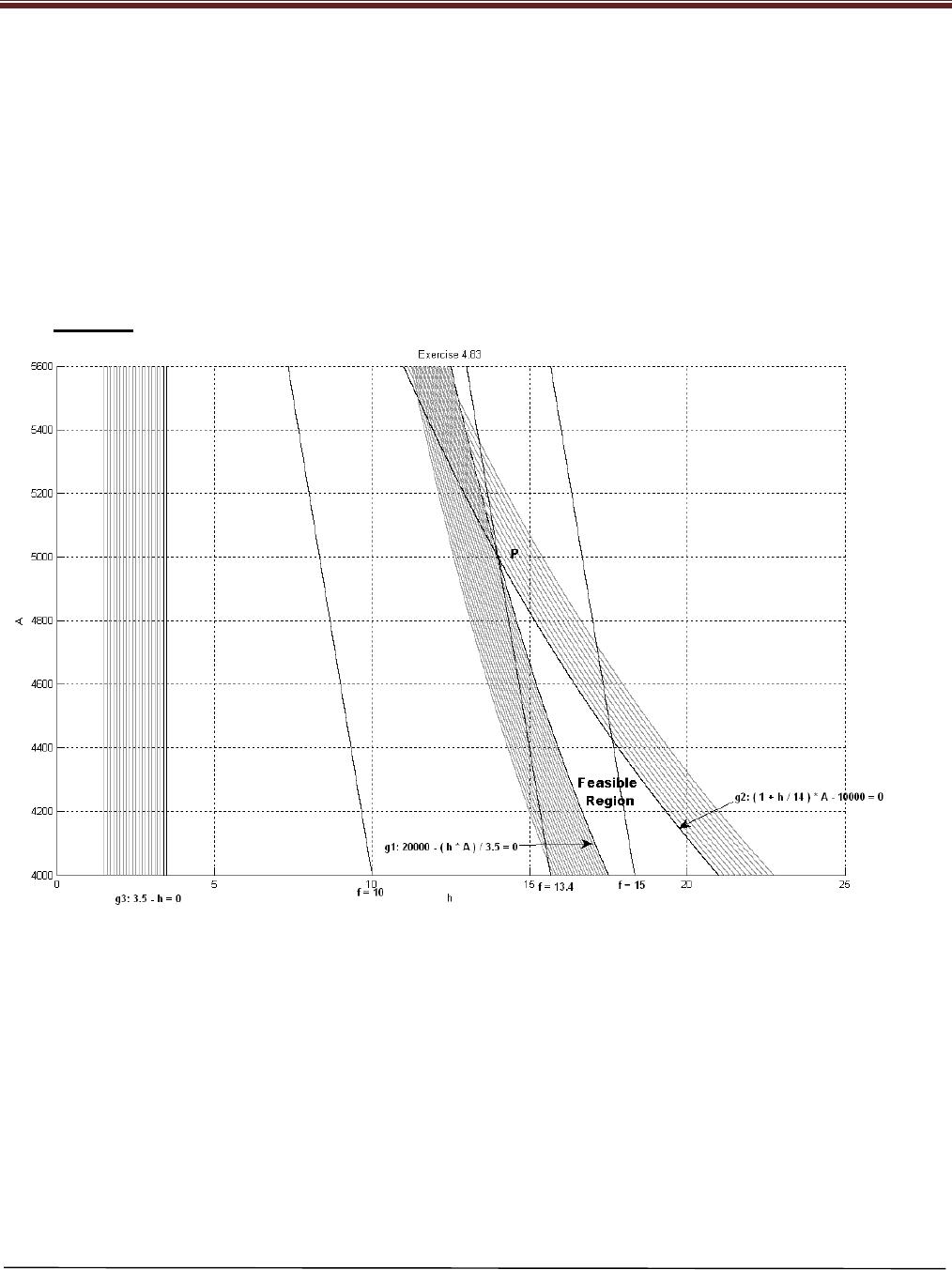
Solution

Chapter 4 Optimum Design Concepts: Optimality Conditions
Referring to the formulation in Exercise 2.1 we have
Minimize
1
0 6 0 001 , subject to: g 20,000 3 5 0;f h A hA=+ =−≤.. .
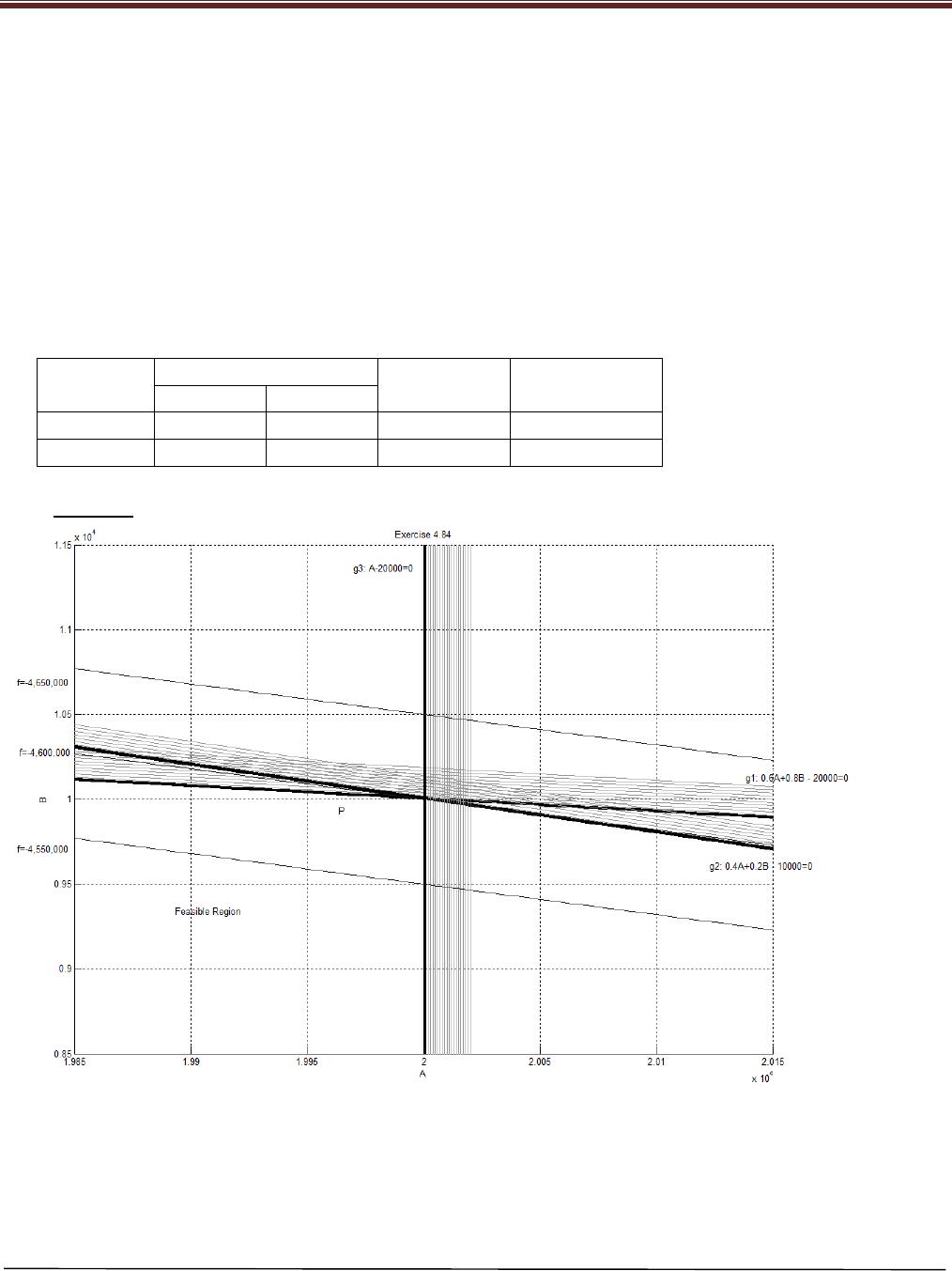
f = 13.4 mil. dollars. The solution can be verified graphically. It is seen that the point obtained

Chapter 4 Optimum Design Concepts: Optimality Conditions
MATLAB Code for Exercise 4.83
clear all
g3=3.5–h;
g4=–A;
cla reset
axis ([0 25 4000 5600])
xlabel(‘h’),ylabel(‘A’)
cv3=[0:0.1:2];
const3=contour(h,A,g3,cv3,‘g’);
cv3=[0 0.1];
const3=contour(h,A,g3,cv3,‘k’);
cv4=[0:1:5];
Arora, Introduction to Optimum Design, 4e
4-57
4.84__________________________________________________________________________
A refinery has two crude oils:
1. Crude A costs $120/barrel (bbl) and 20,000bbl are available.
2. Crude B costs $150/bbl and 30,000 are available.
The company manufactures gasoline and lube oil from the crudes. Yield and sale price barrel of the
product and markets are shown in Table E2.2. How much crude oils should the company use to
maximize its profit? Formulate the optimum design problem.
Table E2.2 Data for Refinery Operation
Product
Yield/bbl
Sale Price
per bbl ($)
Market (bbl)
Crude A
Crude B
Gasoline
0.6
0.8
200
20,000
Lube oil
0.4
0.2
450
10,000
Solution

Chapter 4 Optimum Design Concepts: Optimality Conditions
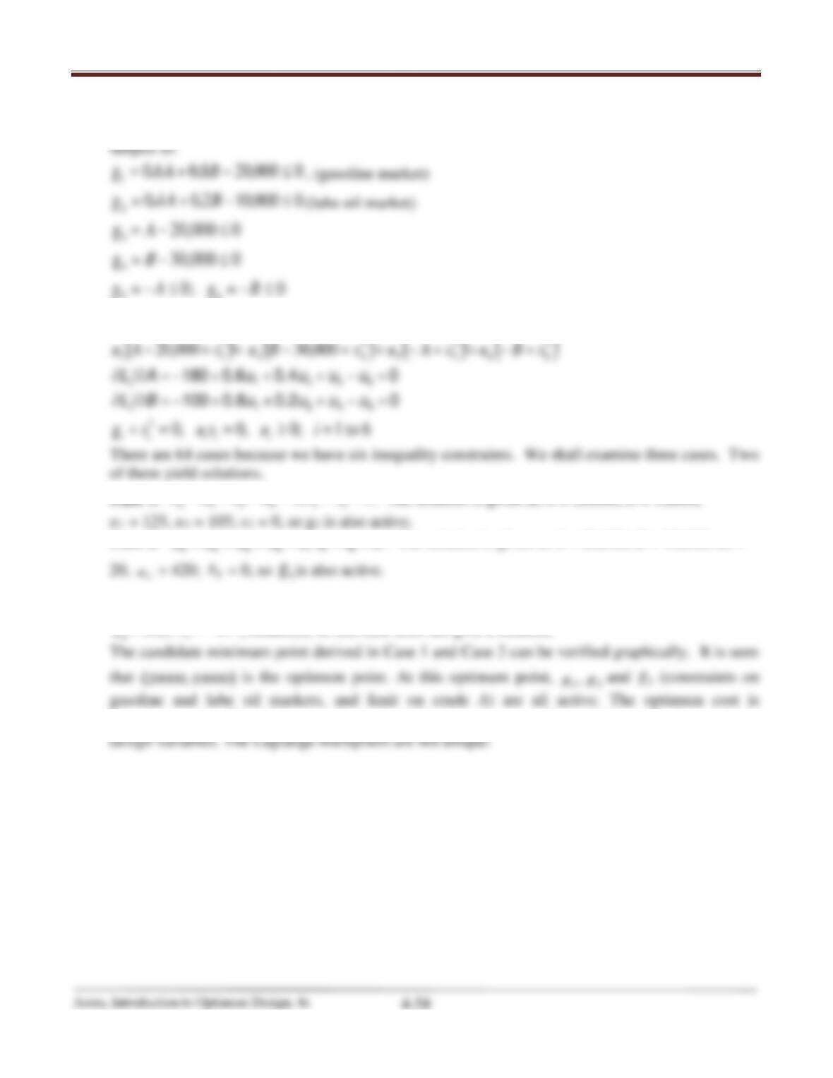
Referring to the formulation in Exercise 2.2, we have
Minimize
180 100f =– A- B
56
( ) ( )
( )
22
1 12 2
180 100 0 6 0 8 20,000 0 4 0 2 10,000=− − + + − ++ + − + +.. ..L A B u A B su A B s
Case 1.
0 ,0
====== ssuuuu
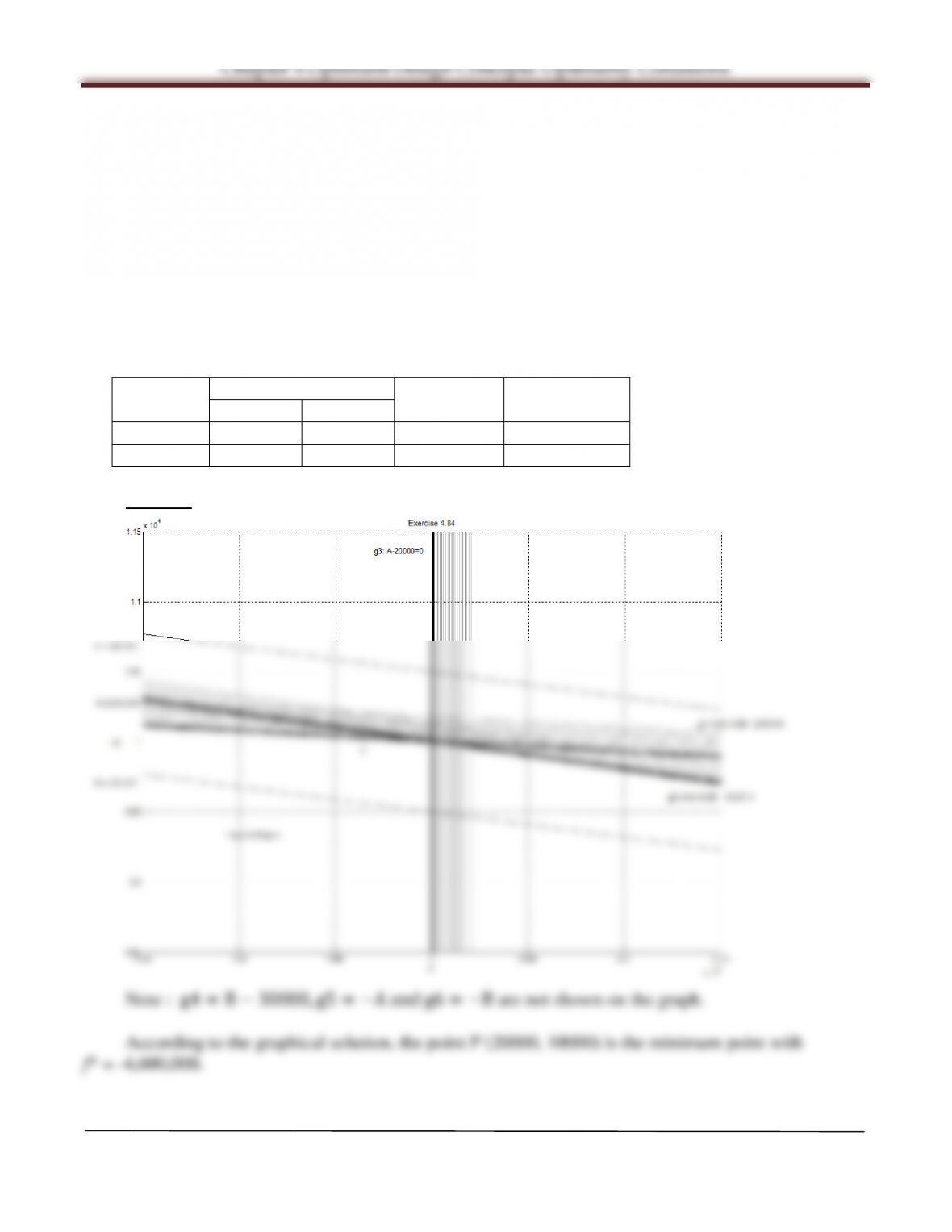
. The solution is given as A = 20,000, B = 10,000,
Case 2.
0, 0u u u u ss= = = = = =
. The solution is given as A = 20,000, B = 10,000, u1 =
Case 3.
0 ,0
326541
====== ssuuuu
. The solution is given as A = 20,000, B = 10,000,
= 500,
(violation); so this case does not give a solution.
-4,600,000.=f
. The optimum point is irregular, since there are three active constraints and two

Chapter 4 Optimum Design Concepts: Optimality Conditions
MATLAB Code for Exercise 4.84
clear all
[A,B]=meshgrid(19850:10:20150,8500:10:11500);
f=–180*A–100*B;
g1=0.6*A+0.8*B–20000;
cv1=[0:15:150];
const1=contour(A,B,g1,cv1,‘g’);
cv1=[0:1:10];
const1=contour(A,B,g1,cv1,‘k’);
cv2=[0:4:30];
const4=contour(A,B,g4,cv4,‘k’);
cv5=[0:1:5];
const3=contour(A,B,g5,cv5,‘g’);
cv5=[0];
const5=contour(A,B,g5,cv5,‘k’);
Arora, Introduction to Optimum Design, 4e
4-60
4.85________________________________________________________________________________
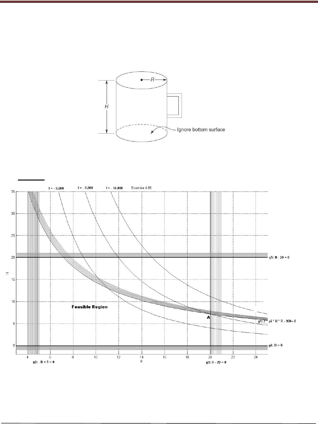
Design a beer bug, shown in Fig. E2.3, to hold as much beer as possible. The height and radius of
the mug should be not more than 20 cm. The mug must be at least 5cm in radius. The surface area of
the sides must not be greater than 900 cm2 (ignore the area of the bottom of the mug and ignore the
mug handle – see figure). Formulate the optimum design problem.
FIGURE E2.3 Beer mug.
Solution
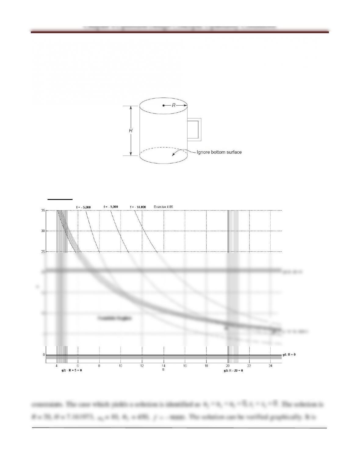
According to the graphical solution, the point A (20, 7.161973) is minimum point.
Referring to the formulation in Exercise 2.3, we have 32 cases because we have five inequality