Chapter 3 Graphical Optimization and Basic Concepts
MATLAB Code
%Exercise 3.10
%Create a grid from –1 to 7 with an increment of 0.01 for the variables x1 and x2
[x1,x2]=meshgrid(–1:0.01:2.0, –0.5:0.01:2.0);
%Enter functions for the minimization problem
f=3*x1+6*x2;
text(0.25,1.75,‘g2’)
text(1.5,1.,‘g3’)
text(0,0.6,‘Feasible Region’)
fv=[–3 –0.5 3 6]; %Defines contours for the minimization function
Arora, Introduction to Optimum Design, 4e
3-22
3.11 ________________________________________________________________________________
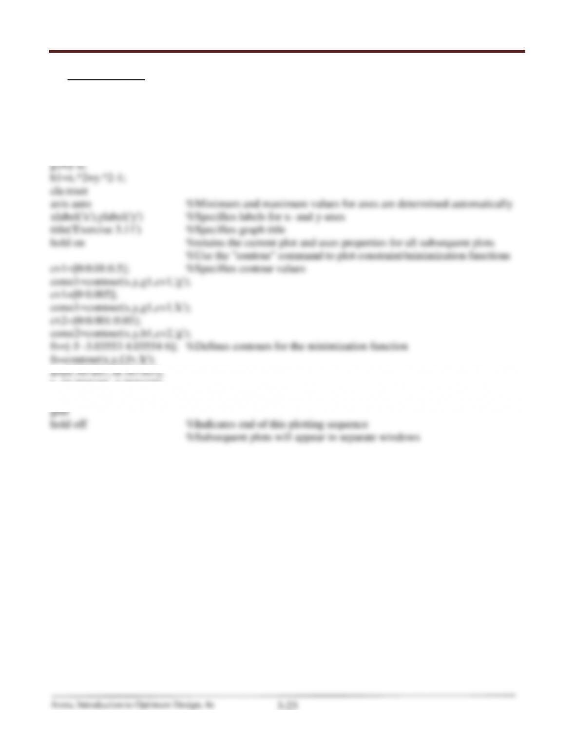
(,)= 22+2−2 −3 − 2
subject to − ≤ 0
2+2−1 = 0
Solution
(,)= 22+2−2 −3 − 2
Chapter 3 Graphical Optimization and Basic Concepts
MATLAB Code
%Exercise 3.11
%Create a grid from -2 to 4 with an increment of 0.05 for the variables x and y
[x,y]=meshgrid(-2:0.05:4, -2:0.05:4);
%Optimization and constraint functions
f=2*x.^2+y.^2-2*x.*y-3*x-2*y;
b=[0.707107,-0.707107];
plot(a,b,’.k’); %Plots points a and b in black
Chapter 3 Graphical Optimization and Basic Concepts
Arora, Introduction to Optimum Design, 4e
3-24
3.12 ________________________________________________________________________________
(,)= 42+ 32−5 −8
subject to += 4
Solution
Chapter 3 Graphical Optimization and Basic Concepts
MATLAB Code
%Exercise 3.12
%Create a grid from -5 to 5 with an increment of 0.005 for the variables x and y
[x,y]=meshgrid(-5:0.005:5, -5:0.005:5);
%Optimization and constraint functions
f=4*x.^2+3*y.^2-5*x.*y-8*x;
Arora, Introduction to Optimum Design, 4e
3-26
3.13 ________________________________________________________________________________
(,)= 92+132+18 −4
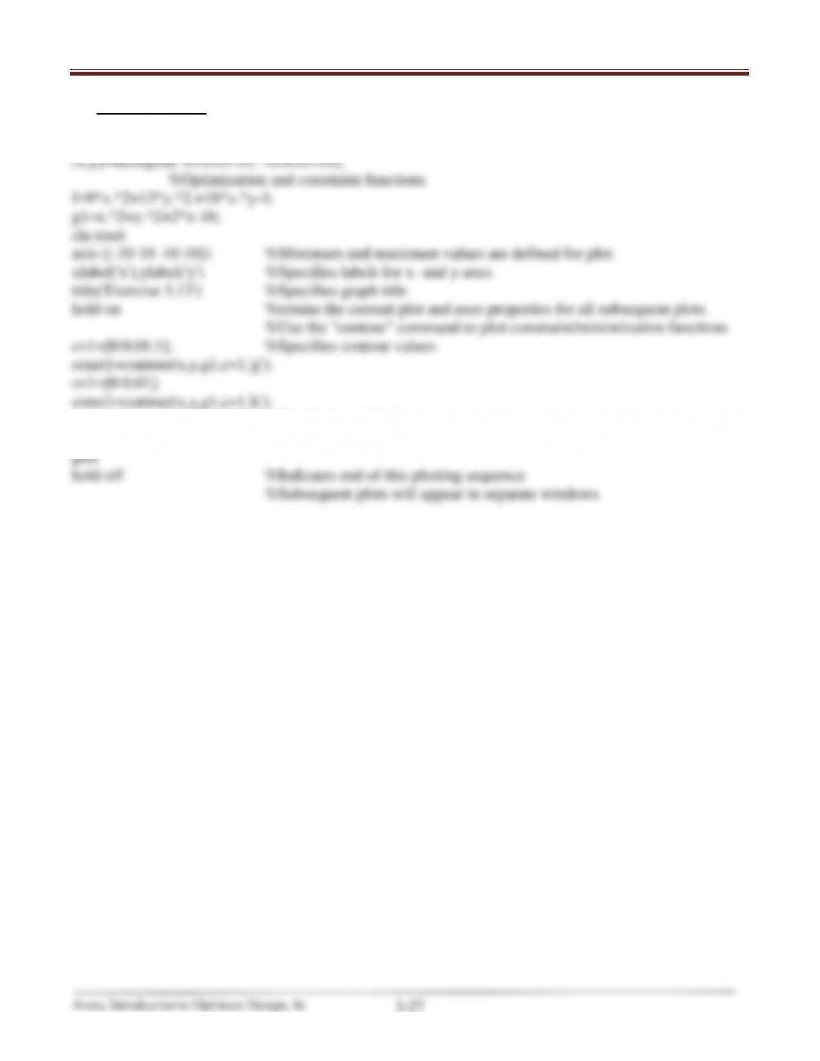
subject to 2+2+ 2=16
Solution
(,)= 92+132+18 −4
Chapter 3 Graphical Optimization and Basic Concepts
MATLAB Code
%Create a grid from -10 to 10 with an increment of 0.05 for the variables x and y
fv=[15.2909 37.8765 244.528 453.1539]; %Defines contours for the minimization function
fs=contour(x,y,f,fv,’b‘);
Chapter 3 Graphical Optimization and Basic Concepts
Arora, Introduction to Optimum Design, 4e
3-28
3.14 ________________________________________________________________________________
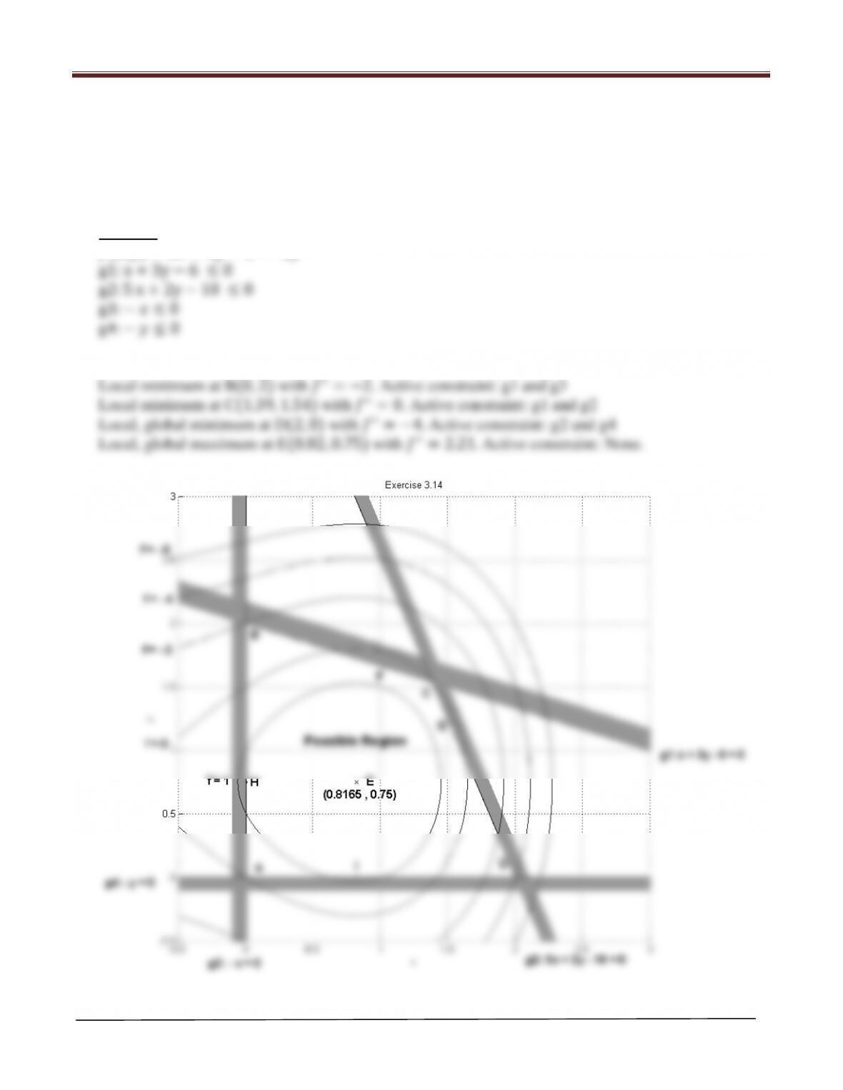
(,)= 2+ 3 − 3−22
subject to + 3 ≤ 6
5+ 2 ≤ 10
, ≥ 0
Solution
(,)= 2+ 3 − 3−22
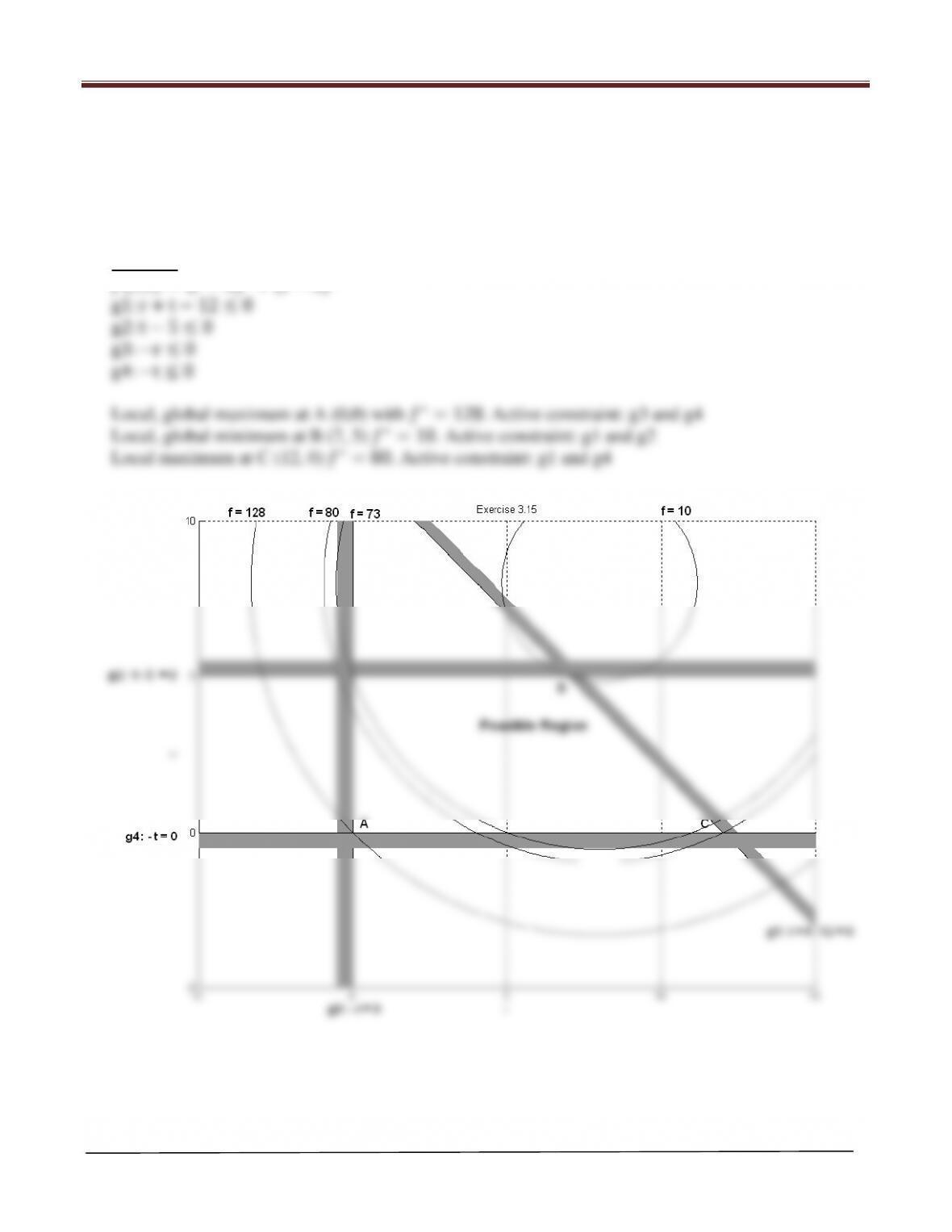
Local minimum at A(0, 0) with ∗= 0. Active constraint: g3 and g4
Chapter 3 Graphical Optimization and Basic Concepts
MATLAB Code
%Create a grid from -1 to 3 with an increment of 0.05 for the variables x and y
[x,y]=meshgrid(-1:0.05:3, -1:0.05:3);
hold on %retains the current plot and axes properties for all subsequent plots
%Use the “contour” command to plot constraint/minimization functions
cv1=[0:0.0005:0.5]; %Specifies contour values
const1=contour(x,y,g1,cv1,’g’);
cv1=[0 0.001];
b=[1.65535,1.23163,0.75,0];
plot(a,b,’.k’); %Plots points a and b in black
d=[0.75];
plot(c,d,’x’); %Plots points c and d
Chapter 3 Graphical Optimization and Basic Concepts
Arora, Introduction to Optimum Design, 4e
3-30
3.15 ________________________________________________________________________________
(,)= ( − 8)2+ ( − 8)2
subject to 12 ≥ +
≤ 5
, ≥ 0
Solution
(,)= ( − 8)2+ ( − 8)2
Chapter 3 Graphical Optimization and Basic Concepts
MATLAB Code
%Create a grid from -5 to 15 with an increment of 0.05 for the variables r and t
[r,t]=meshgrid(-5:0.05:15, -5:0.05:10);
hold on %retains the current plot and axes properties for all subsequent plots
%Use the “contour” command to plot constraint/minimization functions
cv1=[0:0.01:0.5]; %Specifies contour values
const1=contour(r,t,g1,cv1,’g’);
cv1=[0 0.001];
const4=contour(r,t,g4,cv4,’g’);
cv4=[0 0.001];
const4=contour(r,t,g4,cv4,’k’);
fv=[10 73 80 128]; %Defines contours for the minimization function
fs=contour(r,t,f,fv,’b’);