Chapter 3 Graphical Solution Method and Basic Optimization Concepts
Arora, Introduction to Optimum Design, 4e
3-41
3.21________________________________________________________________________________
Solve the rectangular beam problem of Exercise 2.17 graphically for the following data: M = 80 kN
⋅
m, V=150 kN, σa=8 MPa, and τa=3 MPa.
Solution
Rewrite the formulation of Exercise 2.17, and substitute the following data:
6
5
4
5
g0
d
=−≤
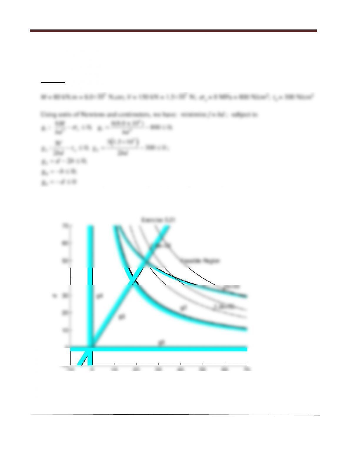
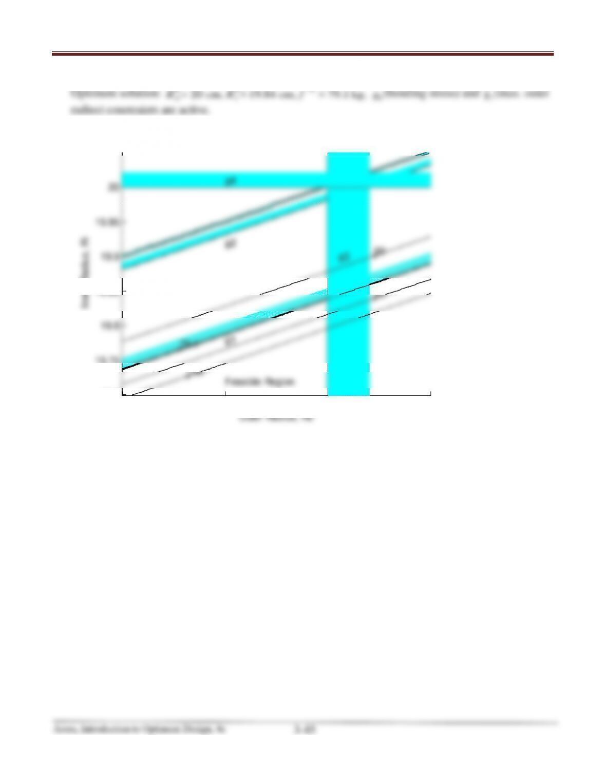
Optimum solution: b
∗
=
24.66 cm, d
∗
=
49.32 cm, f
∗
=
1216 cm2; g1 (bending stress) and g3
(depth- ratio) constraints are active.
0
10
20
30
40
50
60
70
b
d
Exercise 3.21
g1
g2
g3
g5
g4
Feasible Region
1.2e+03
1.5e+03
2e+03
Chapter 3 Graphical Solution Method and Basic Optimization Concepts
MATLAB Code
%Exercise 3.21
%Create a grid from –10 to 70 with an increment of 0.1 for the variables x1 and x2
g3=0.5.*d–b;
g4=–b;
g5=–d;
cla reset
axis auto
const1=contour(b,d,g1,cv22,‘c’);
const2=contour(b,d,g2,cv1,‘k’,‘Linewidth’,4);
const2=contour(b,d,g2,cv22,‘c’);
text(40,23,‘g2’)
const3=contour(b,d,g3,cv1,‘k’,‘Linewidth’,4);
Arora, Introduction to Optimum Design, 4e
3-43
3.22 ________________________________________________________________________________
Solve the cantilever beam problem of Exercise 2.23 graphically for the following data:
P = 10 kN; l = 5.0 m; modulus of elasticity, E = 210 GPa; allowable bending stress σa= 250 MPa;
allowable shear stress, τa= 90 MPa; mass density, ρ = 7850 kg/m3 ; R0
≤
20.0 cm; Ri
≤
20.0 cm.
Solution
Using kg, N and cm as units
Given Data: (this data will change if different units are used)
oi
Maximum bending stress:
Maximum shearing stress:
3−
3); = 2(− )
=
3(
In addition, it must be ensured that > which can be imposed as a constraint on the wall
thickness as ≥ with as, say 0.1 cm.
Referring to Exercise 2.23 and the given data, the problem is formulated in terms of the design
( )
144
oi
RR
−
Chapter 3 Graphical Solution Method and Basic Optimization Concepts
Arora, Introduction to Optimum Design, 4e
3-44
( )
( )
22
o oi i
244
oi
4
g = τ ; or
3πa
P R RR R
RR
++
≤
−
( )
( )
( )
42 2
o oi i
244
oi
4.0 10
g = 9000;
3π
R RR R
RR
× ++
≤
−
or
( )
( )
22
o oi i
244
oi
4244.13
g 9000 0;
R RR R
RR
++
= −≤
−
3o
4i
5o
6i
g 20 0;
g 20 0;
g 0;
g0
R
R
R
R
=−≤
=−≤
=−≤
=−≤
FORMULATION 2: Using Intermediate Variables
Step 4: Optimization Criterion
Optimization criterion is to minimize mass of hollow tube, and the cost function is defined as
Step 5: Formulation of Constraints
g1 : bending stress should be smaller than the allowable bending stress; ≤
g2 : shear stress smaller than allowable shear stress: ≤
2= − ≤0
Chapter 3 Graphical Solution Method and Basic Optimization Concepts
∗∗ ∗
19.9 19.95 20 20.05
19.7
19.75
19.8
19.85
19.9
19.95
20
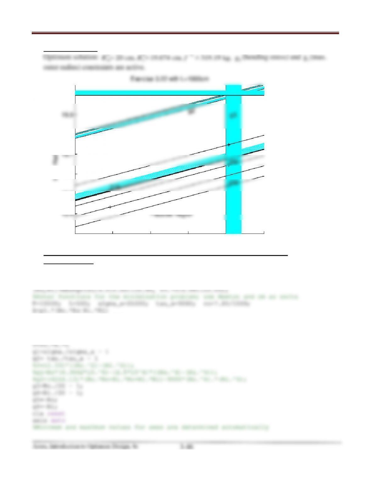
Exercise 3.22
Outer Radius, Ro
Inner Radius, Ri
g1
g2
g3
g4
Feasible Region
60
79.1
90
100
Chapter 3 Graphical Solution Method and Basic Optimization Concepts
With L = 1000cm
∗∗ ∗
MATLAB Code
%Exercise 3.22
%Create a grid
I=0.25.*pi.*(Ro.^4–Ri.^4)
sigma=P.*L.*Ro./I
tau=P.*(Ro.*Ro+Ro.*Ri+Ri.*Ri)./(3.*I)
19.8 19.85 19.9 19.95 20 20.05
19.3
19.4
19.5
19.6
19.7
19.8
19.9
20
Exercise 3.22 with L=1000cm
Outer Radius, Ro
Inner Radius, Ri
g1
g2 g3
g4
Feasible Region
250
319
350
400
450
Chapter 3 Graphical Solution Method and Basic Optimization Concepts
title(‘Exercise 3.22’)
xlabel(‘Outer Radius, Ro’),ylabel(‘Inner Radius, Ri’) %Specifies labels for x–
and y–axes
text(19.95,19.92,‘g2’)
text(19.95,20.01,‘g4’)
text(6,0.5,‘g5’)
text(19.95,19.72,‘Feasible Region’)
fv=[60 79.1 90 100]; %Defines contours for the minimization function
fs=contour(Ro,Ri,f,fv,‘k–‘); %’k’ specifies black dashed lines for function
contours
I=0.25.*pi.*(Ro.^4–Ri.^4)
sigma=P.*L.*Ro./I
tau=P.*(Ro.*Ro+Ro.*Ri+Ri.*Ri)./(3.*I)
t=Ro–Ri
Chapter 3 Graphical Solution Method and Basic Optimization Concepts
g6=–Ri;
cla reset
axis auto
text(19.95,19.92,‘g2’)
text(19.95,20.01,‘g4’)
text(6,0.5,‘g5’)
text(19.9,19.4,‘Feasible Region’)
fv=[250 319.185 350 400 450]; %Defines contours for the minimization function
Arora, Introduction to Optimum Design, 4e
3-49
3.23________________________________________________________________________________
For the minimum mass tubular column design problem formulated in Section 2.7, consider the
following data: P = 50 kN; l = 5.0 m; modulus of elasticity, E= 210 GPa; allowable stress, σa= 250
MPa; mass density, = 7850 kg/m3.
Treating mean radius R and wall thickness t as design variables, solve the design problem
graphically imposing an additional constraint R/t
≤
50. This constraint is needed to avoid local
crippling of the column. Also impose the member size constraints as
0.01≤ R ≤ 1.0 m; 5 ≤ t ≤ 200 mm
Solution
Referring to Formulation 1 of Section 2.7.1 and imposing an additional constraint R/t
≤
50, we
summarize the formulation as follows:
max
Use Newtons and millimeters as units.
6
≤
≤
4
5
Substitute the given data into f, g1 and g2:
4
6
Chapter 3 Graphical Solution Method and Basic Optimization Concepts
3
g 50 0
R
t
=−≤
4
g 10 0R= −≤
5
g 1000 0R=−≤
6
g5 0t= −≤
7
g 200 0t=−≤
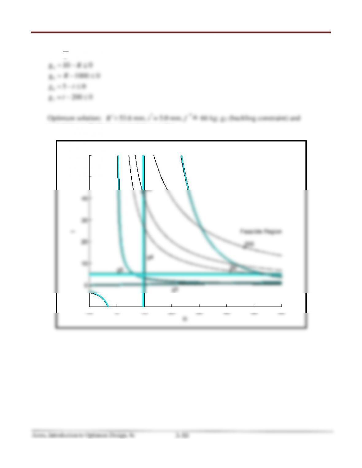
Optimum solution:
R∗=
53.6 mm, t
∗
= 5.0 mm, f
=
∗
66 kg; g2 (buckling constraint) and
g6 (minimum thickness constraint) are active.
-10 010 20 30 40 50 60
-10
0
10
20
30
40
50
60
R
t
g1
g2
g3
g4
g6
Feasible Region
66
100
200
Exercise 3.23
Chapter 3 Graphical Solution Method and Basic Optimization Concepts
MATLAB Code
f=0.2466*R.*t;
g1=7957.7-250*R.*t;
g2=5*10^4-0.06511*(R.^3).*t;
g3=R-50*t;
g4=10-R;
cv11=[0.01:0.01:0.5];
const1=contour(R,t,g1,cv11,’c’);
const2=contour(R,t,g2,cv1,’k’,’Linewidth’,3);
const2=contour(R,t,g2,cv11,’c’);
text(27,58,’g2′)
const6=contour(R,t,g6,cv11,’c’);
text(0,7,’g6′)
const7=contour(R,t,g7,cv1,’k’,’Linewidth’,3);
const7=contour(R,t,g7,cv11,’c’);
text(6,200,’g7′)
Chapter 3 Graphical Solution Method and Basic Optimization Concepts
3.24________________________________________________________________________________
For Exercise 3.23, treat outer radius 0 and inner radius as design variables, and solve the design
problem graphically. Impose the same constraints as in Exercise 3.23.
Solution
Referring to Formulation 2 of Section 2.7.2 and Exercise 3.23, the problem is formulated as
f =
( )
22
oi
πlR R−
ρ
;
Pσ
( )
oi
oi
10 1000
5 m0. m
RR
≤ −≤
Use Newtons and millimeters as units, and the data given in Exercise 3.23:
f =
( )
( )
( ) ( )
6 22 22
oi oi
π 7.85 10 5000 0.1233RR RR
−
× −= −
( )
122
oi
15915.5
g 250 0
RR
= −≤
−
;
( ) ( )
( )
( ) ( )
3 5 44
oi
4
22
4 44
2 oi
π 2.1 10
g : 5.0 10 ; or
16 5000
g 5 10 0.016278 0
RR
RR
×−
×≤
=×− −≤
)
( )
( )
oi
3
oi
4 oi
5 oi
g 50 0;
2
g 5 0;
g 200 0
RR
RR
RR
RR
+
= −≤
−
=− + +≤
= −− ≤
g6
( )
oi
0.5 1000 0RR=− +− ≤
;
g7
( )
oi
0.5 1000 0RR= +− ≤
Chapter 3 Graphical Solution Method and Basic Optimization Concepts
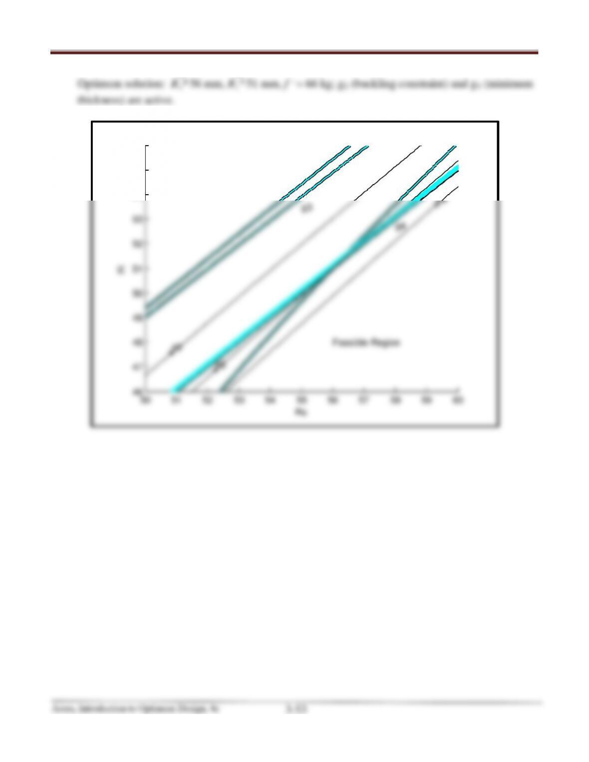
Optimum solution: R
=
∗
o
56 mm, R
=
∗
i
51 mm, f
∗
= 66 kg; g2 (buckling constraint) and g4 (minimum
thickness) are active.
50 51 52 53 54 55 56 57 58 59 60
46
47
48
49
50
51
52
53
54
55
56
Ro
Ri
g1
g2
g3
g4
Feasible Region
40
66
80
Exercise 3.24
Chapter 3 Graphical Solution Method and Basic Optimization Concepts
MATLAB Code
[Ro,Ri]=meshgrid(50:0.1:60, 46:0.1:56);
%Enter functions for the minimization problem
f=0.1233*(Ro.^2-Ri.^2);
g1=15915.5-250*(Ro.^2-Ri.^2);
g2=5*10^4-0.016278*(Ro.^4-Ri.^4);
g3=(Ro+Ri)-100*(Ro-Ri);
g4=5–Ro+Ri;
cv11=[0.01:0.01:0.2];
const1=contour(Ro,Ri,g1,cv11,’c’);
const2=contour(Ro,Ri,g2,cv1,’k’,’Linewidth’,3);
const2=contour(Ro,Ri,g2,cv11,’c‘);
text(59,55.5,’g2′)
const6=contour(Ro,Ri,g6,cv11,’c’);
text(0,7,’g6′)
const7=contour(Ro,Ri,g7,cv1,’k’,’Linewidth’,3);
const7=contour(Ro,Ri,g7,cv11,’c’);
text(6,200,’g7′)
Arora, Introduction to Optimum Design, 4e
3-55
3.25 ________________________________________________________________________________
Formulate the minimum mass column design problem of Section 2.7 using a hollow square cross
section with outside dimension w and thickness t as design variables. Solve the problem
graphically using the constraints and the data given in Exercise 3.23.
Solution
For a hollow square cross-section with outside dimension w and thickness t, the cross-sectional
area and moment of inertia are
44
4
4
2
22
22
wt w wt
w
Referring to Section 2.7 and Exercise 3.23, the problem is formulated as
f =
( )
2
44l wt t−
ρ
2
Use Newtons and millimeters as units, and the data given in Exercise 3.23:
2
6
2
2

Chapter 3 Graphical Solution Method and Basic Optimization Concepts
Arora, Introduction to Optimum Design, 4e
3-56
Chapter 3 Graphical Solution Method and Basic Optimization Concepts
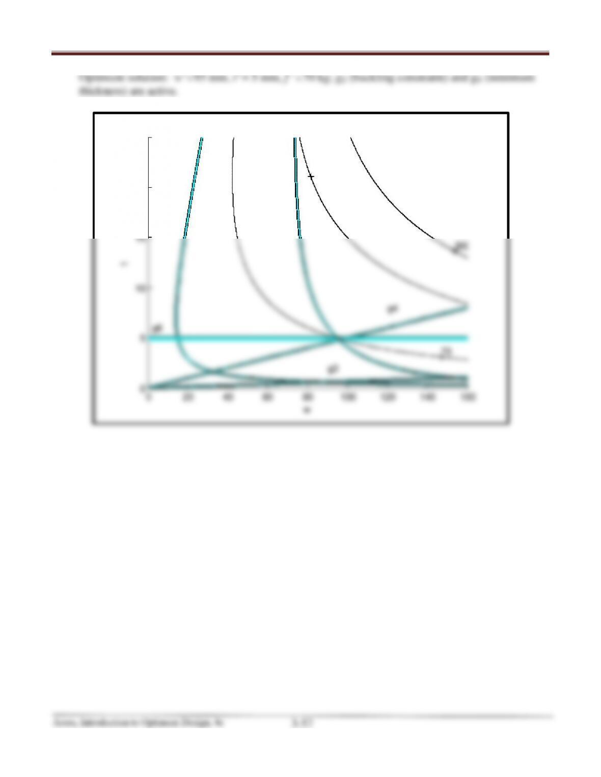
Optimum solution: w
=
∗
93 mm, t
∗
= 5 mm, f
=
∗
70 kg; g2 (buckling constraint) and g6 (minimum
thickness) are active.
020 40 60 80 100 120 140 160
0
5
10
15
20
25
w
t
g1 g2
g3
g4
g6
Feasible Region
70
200
300
Exercise 3.25
Chapter 3 Graphical Solution Method and Basic Optimization Concepts
MATLAB Code
f=0.157*(w.*t-t.^2);
g1=12500-250*(w.*t-t.^2);
g2=5*10^4-(1.7271*10^-3)*(w.^4-(w-2*t).^4);
g3=w-151*t;
g4=20*t-w;
cv11=[0.01:0.01:0.2];
const1=contour(w,t,g1,cv11,’c’);
const2=contour(w,t,g2,cv1,’k’,’Linewidth’,3);
const2=contour(w,t,g2,cv11,’c’);
text(76,20,’g2′)
const6=contour(w,t,g6,cv11,’c’);
text(2,6,’g6′)
const7=contour(w,t,g7,cv1,’k’,’Linewidth’,3);
const7=contour(w,t,g7,cv11,’c’);
text(6,200,’g7′)
Chapter 3 Graphical Solution Method and Basic Optimization Concepts
Arora, Introduction to Optimum Design, 4e
3-59
3.26 ________________________________________________________________________________
Consider the symmetric (member are identical) case of the two-bar truss problem discussed in
Section 2.5 with the following data: W = 10kN ; = 30°; height h = 1.0m; span s = 1.5m;
allowable stress = 250MPa; modulus of elasticity, E = 210GPa.
Formulate the minimum mass design problem with constraints on member stresses and bounds
on design variables. Solve the problem graphically using circular tubes as members.
Solution
Design variables: D
o
= outer diameter of the tube; D
i
= inner diameter of the tube
22 22
oi oi
Constraints:
s
θ
s
θ
22
22
22
oi
where W = 10 kN,
θ
= 30°,
ρ
= 7850 kg/m3, h = 1.0 m, s = 1.5 m,
a
σ
= 250 MPa
( ) ( )
22
2
2 1 0.75 1.25l hs=+=+ =
For 0°
≤≤
θ
90°; sin
≥
θ
0, cos
≥
θ
0;
(sin
2coshs+
θθ
)
≥
(sin
h−
θ
2cos
s
θ
);
(sin
2coshs+
θθ
)
≥
(2cos
s−
θ
sin
h
θ
)
We could drop g2 and g3, since they are redundant.
Use kN and cm as the units; substitute the constants into f and g1,
f =
( )
( ) ( )
22 22
oi oi
π 2 196.3l DD DD−= −
( )( )
( ) ( )
22
1 oi
g 2 10 125 0.005 2cos30 150 25 0;DD
= + − −≤
π
ο
or
( )
22
1 oi
2o
3i
4 oi
g 13.1675 25 0;
g : 0;
g : 0;
g : 0
DD
D
D
DD
= − −≤
−≤
−≤
− +≤
Chapter 3 Graphical Solution Method and Basic Optimization Concepts