Chapter 3 Graphical Solution Method and Basic Optimization Concepts
Arora, Introduction to Optimum Design, 4e
3-139
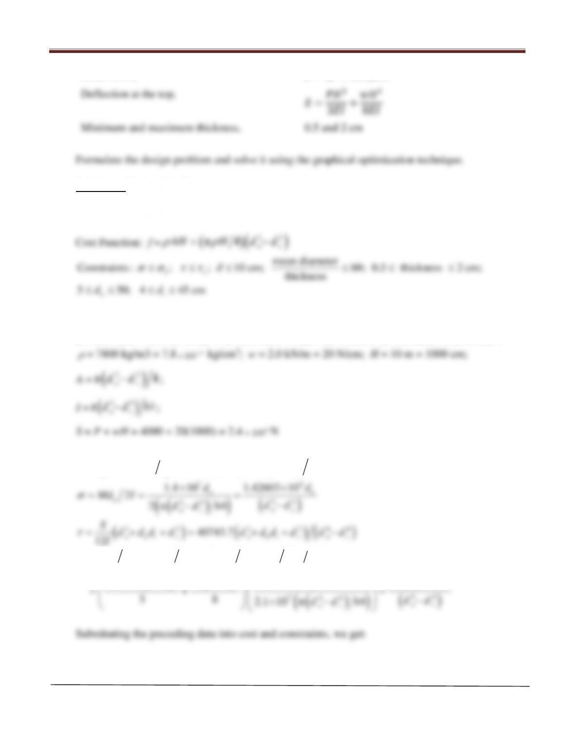
Shear stress,
=(+),kN
Deflection at the top,
=3
3 +4
8
Minimum and maximum thickness,
0.5 and 2 cm
Formulate the design problem and solve it using the graphical optimization technique.
Solution: Design of a flag pole-
Design Variables: do = outer diameter of the flag pole; di = inner diameter of the flag pole
22
oi
5 50; 4 45 cm
dd
≤≤ ≤≤
Use units of Newtons and centimeters. The pertinent data are given as : P = 4.0 kN = 4000 N
E = 210 GPa =
7
1012 ×.
N/cm2;
b
σ
= 165 MPa =
4
10651 ×.
N/cm2;
s
τ
= 50 MPa = 5000 N/cm2;
ρ
= 7800 kg/m3 = 7.8
3
10−
×
kg/cm3; w = 2.0 kN/m = 20 N/cm; H = 10 m = 1000 cm;
A =
( )
22
oi
π4dd−
;
I =
( )
44
oi
π 64dd−
;
S = P + wH = 4000 + 20(1000) = 2.4
4
10×
N
( )
( ) ( )
2
23 7
2 4 10 1000 20 1000 2 1.4 10 N.cmM PH wH=+=× + =×
( )
( )
( )
78
oo
o44
44
oi
oi
1.4 10 1.42603 10
2
2π 64
dd
Md I dd
dd
σ
××
= = = −
−
( ) ( ) ( )
22 2244
o oi i o oi i o i
40743.7
12
Sd dd d d dd d d d
I
τ
= ++= ++ −
( )
( )
( ) ( )
( )
( )
( )
3 4 34
34 6
44
7 44
oi
oi
3 8 3 81
4 1000 1000 20 1000 1 3.71867 10
38
2.1 10 π 64
PH EI wH EI PH wH EI
dd
dd
δ
=+=+
××
=+=
−
×−
Chapter 3 Graphical Solution Method and Basic Optimization Concepts
( )
(
)
( )
( )
( ) ( )
( )
( ) ( )
( )
–3 22 22
oi oi
8 44 4
1 o oi
2 2 44
2 o oi i o i
6 44
3 oi
π 4 7.8 10 1000 6.12611 , kg
g 1.42603 10 1.65 10 0 (bending stress)
g 40743.7 5000 0 (sheer stress)
g 10 3.71867 10 10 0 (top deflectio
b
s
f dd dd
d dd
d dd d d d
dd
σσ
ττ
δ
= × −= −
=−= × − − × ≤
=−= + + − − ≤
=−= × − −≤
( ) ( )
( )
( )
4 oi oi
5 oi
6 oi
7o
8o
9i
10 i
n)
g 60 0 (diameter-thickness ratio)
g 2 2 0 (maximum thickness)
g 0.5 2 0 (minimum thickness)
g 50 0;
g 5 0;
g 45 0;
g4 0
dd dd
dd
dd
d
d
d
d
= + − −≤
= − −≤
=−− ≤
=−≤
=−≤
=−≤
=−≤
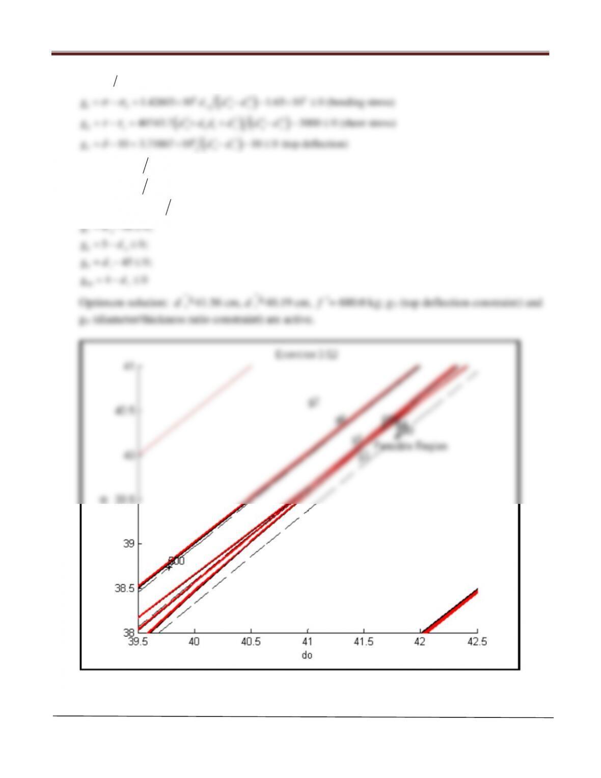
∗=
∗
Chapter 3 Graphical Solution Method and Basic Optimization Concepts
MATLAB Code: 3.52
[do,di]=meshgrid(39.5:0.5:42.5,38:0.5:41);
g1=1.42603*10^8*do./(do.^4-di.^4)-1.65*10^4;
g2=40743.7*(do.^2+do.*di+di.^2)./(do.^4-di.^4)-5000;
g3=3.71867*10^6./(do.^4-di.^4)-10;
g6=0.5-(do-di)/2;
g7=do-50;
g8=5-do;
g9=di-45;
text(41.4,40.18,’g1′)
cv2=(0:0.1:20);
cv22=(20:1:500);
text(41.45,40,’g3′)
cv4=(0.0:0.01:0.3);
text(41.8,40.35,’g4′)
cv5=(0:0.001:0.01);
cv55=(0.01:.001:.03);
Chapter 3 Graphical Solution Method and Basic Optimization Concepts
const6=contour(do,di,g6,cv6,’k’);
const66=contour(do,di,g6,cv66,’r’);
text(41.25,40.4,’g6′)
cv7=(0:0.001:0.012);
text(49.8,40.37,’g7′)
cv8=(0:0.001:0.012);
text(5.2,40.37,’g8′)
cv9=(0:0.001:0.012);
cv99=(0.012:.001:.04);
text(41.6,40.1,’Feasible Region’)
fv=[500, 680, 800];
Chapter 3 Graphical Solution Method and Basic Optimization Concepts
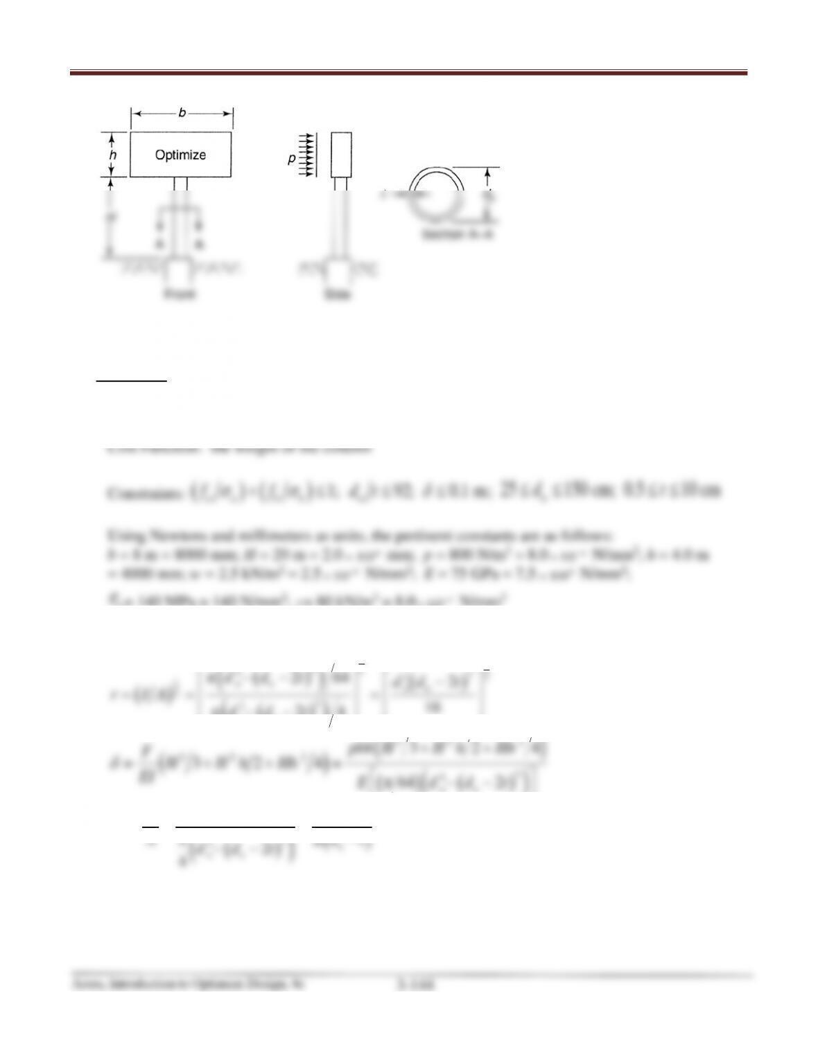
FIGURE E3.53 Sign support column.
Solution: Design of a sign support column-
Design Variables: do = outer diameter of the column; t = wall thickness of the column
Chapter 3 Graphical Solution Method and Basic Optimization Concepts
( )
( ) ( )
( )
o
o
4
4
oo
2
2π 32 2
b
pbh H h wbh d
Md
fIdd t
δ
++
= = −−
( )
( )
( )
( )
22
22 22
2oo oo
22 2
12π23π2
12π
92 16 368
92
a
Ed d t Ed d t
E
HH
Hr
−− −−
σ= = =
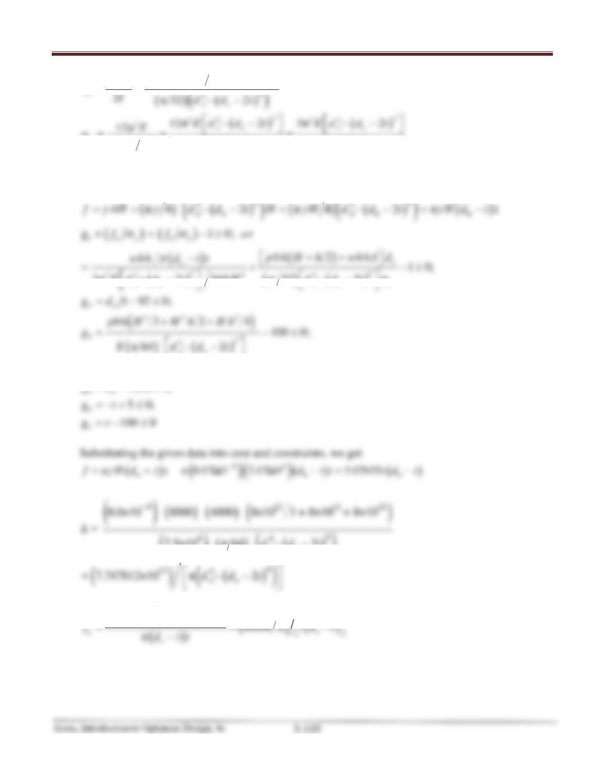
Writing the cost and constraints in terms of design variables, we get
( )
( )
()
( )
( )
()
( )
22
22
oo oo o
π4 2 π 4 2 π tf AH dd tH H dd t Hdt= = −− = −− = −
γγ γ γ
( ) ( )
( )
( )
( )
( ) ( )
( )
( ) ( )
1
24
22 2 4
2o
32 2
34
4
oo
4
5
6
7
g 1 0;
21 0;
3 2 368 32 2
g t 92 0;
324
g 100 0;
π 64 2
g 250 0;
g 1500 0;
g 5 0;
g 100 0
aa bb
o
o
oo oo b
o
o
f f or
pbh H h wbh d
wbh d t t
Ed d t H d d t
d
pbh H H h H h
E dd t
d
d
t
t
σσ
δ
π
π πσ
= + −≤
++
−
= + −≤
+− −−
= −≤
++
= −≤
−−
=−+ ≤
=−≤
=−+ ≤
=−≤
Substituting the given data into cost and constraints, we get
( )
( )( )
( ) ( )
54
o oo
π t = 8.0 10 2.0 10 5.02655f Hd t dtt tdt=−=
γπ
–
‰ ‰- –
( )
( ) ( )
( )
( )
( )
( )
()
( )
( )
()
412 11 10
4
44
oo
4
13 4
oo
–
8.0×10 8000 4000 8×10 3 + 8×10 + 8×10
δ=
7.5×10 π 64 2
= 7.747812×10 π2
dd t
dd t
−−
−−
Chapter 3 Graphical Solution Method and Basic Optimization Concepts
( )( )
( )( ) ( )( )
( )
( ) ( )
3 13
44
o4
4
oo
4
4
oo
2.5 10 7.74781 10
8000 4000 8.0 10 2.0 10 2000
π2
π 32 2
b
d
dd t
f
dd t
−
−
××
× ×+ +
−−
=
−−
( )
( )
( )
( )
10 20
oo
2
44
4 24
oo oo
1.80224 10 1.98344 10
π 2π 2
dd
dd t dd t
××
= +
−− −−
( )
( )
( ) ( )
( )
2
2 42
oo 2
2 52
a oo
2
4
3π 7.5 10 2
σ π 6.542222 10 2
368 2.0 10
dd t
dd t
× +−
= = × +−
×
( ) ( )
( )
( )
( )
( )
7 17
9oo
12
24
24 4
4
o oo oo oo
4.0976487 10 1.435461 10
1.687973 10
g 1.0 0
22 2
dd
td t d d t d d t dd t
××
×
= + + −≤
− +− −−
−−
( )
2o
13
34
4
oo
g 92 0;
2.4662052 10
g 100 0
2
dt
dd t
= −≤
×
= −≤
−−
4o
5o
6
7
g 250 0;
g = 1500 0;
g 5 0;
g = 100 0
d
d
t
t
= −≤
−≤
= −≤
−≤
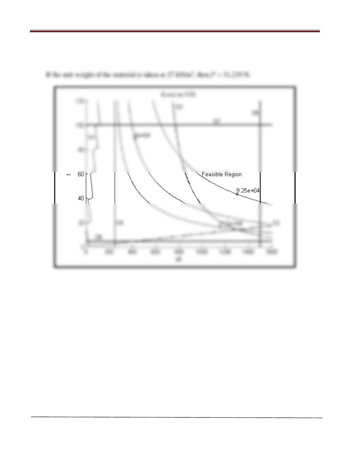
Chapter 3 Graphical Solution Method and Basic Optimization Concepts
Arora, Introduction to Optimum Design, 4e
3-147
Optimum solution:
*
o
d=
1310 mm, t
=
∗
14.2 mm, f
=
∗
92,500 N; g3 (maximum deflection
constraint) and g2 (diameter/thickness ratio constraint) are active.
Chapter 3 Graphical Solution Method and Basic Optimization Concepts
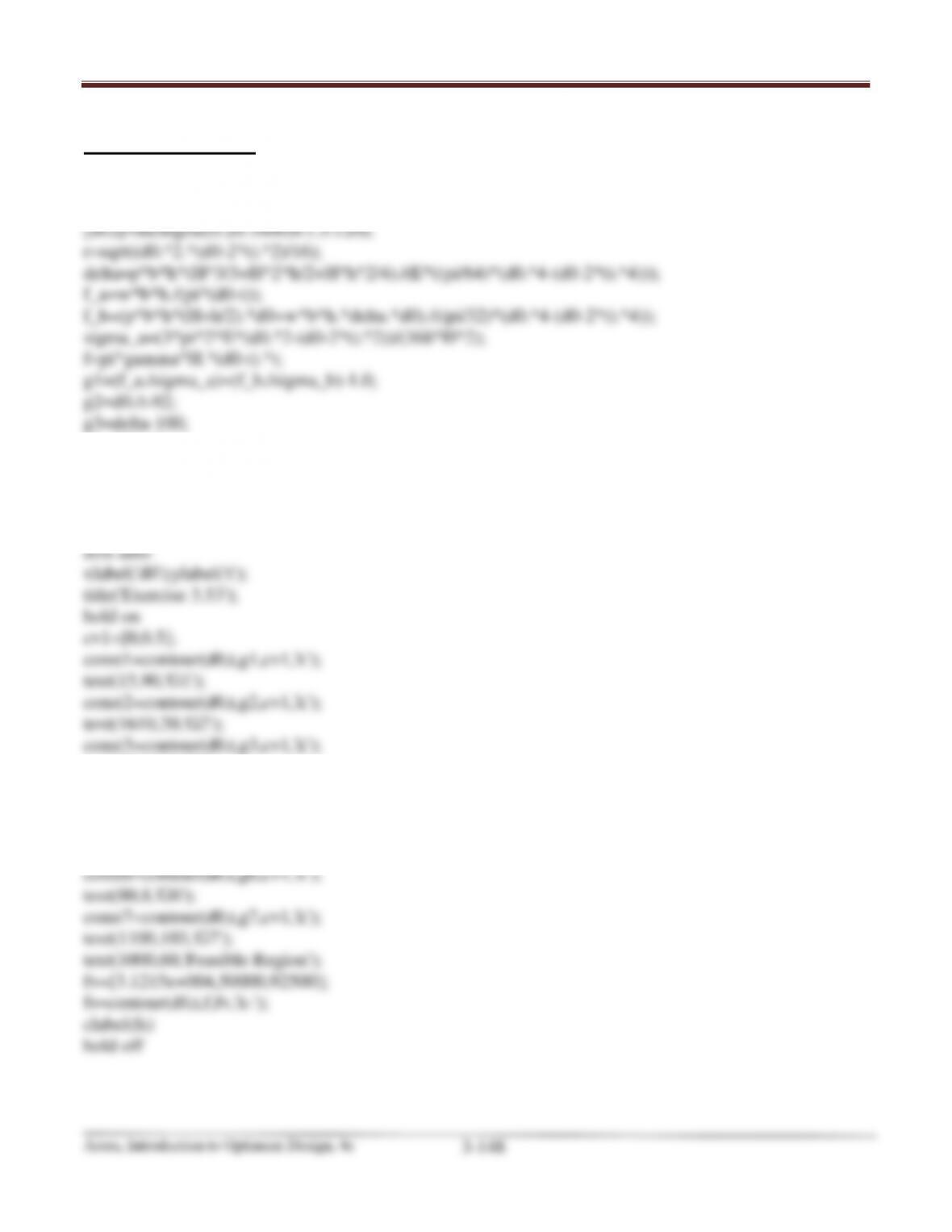
MATLAB Code: 3.53
b=8000;H=20000;p=8*10^(-4);h=4000;w=2.5*10^(-3);E=7.5*10^4;
sigma_b=140;gamma=2.7*10^(-5);
g4=250-d0;
g5=d0-1500;
g6=5–t;
g7=t-100;
cla reset
text(770,115,’G3′);
const4=contour(d0,t,g4,cv1,’k’);
text(260,20,’G4′);
const5=contour(d0,t,g5,cv1,’k’);
text(1430,110,’G5′);
Chapter 3 Graphical Solution Method and Basic Optimization Concepts
Constraints:
( )
1
2
22
122
43
3
g0
π 4 3π
aa a
WH B
Wl H
P
AD DH
+
=−= −= −≤
σσ σ
( ) ( )
( )
1
2
22 2 4
2
cr
2222
3π π 64
Wπ
g= 0
23 3
223
WH B E D
Pl EI
PHH
lHB
+
−= − = − ≤
+
3
4
5
6
g = 500 0;
g 50 0;
g = 50 0;
g 0.5 0
H
H
D
D
−≤
=−+ ≤
−≤
=−+ ≤
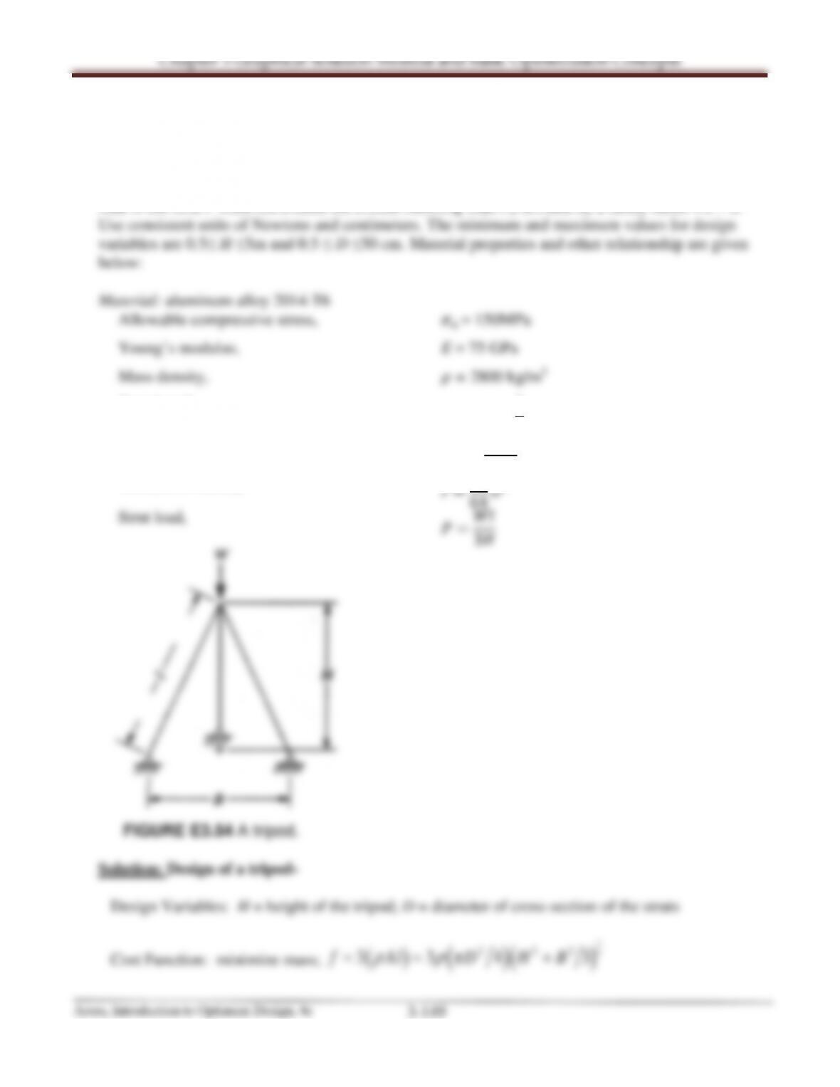
Using units of Newtons and centimeters, the data are calculated as follows:
42 62
3 33 4
150 MPa 1.5 10 N/cm ; 75 GPa 7.5 10 N/cm ;
2800 kg/m 2.8 10 kg/cm ; 1200 mm 120 cm; 60 kN 6.0 10 N
aE
BW
−
==×==×
==×====×
σ
ρ
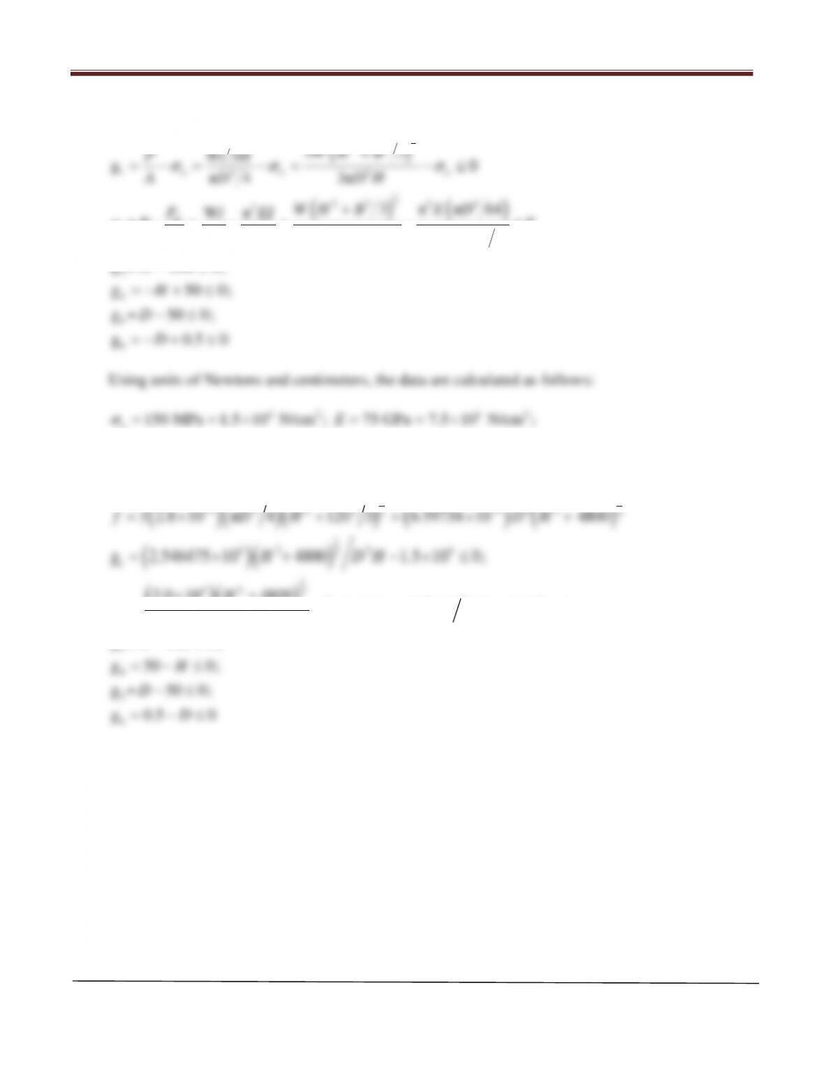
Introducing these constants into the cost and constraints, we get
( )( )( ) ( ) ( )
11
3 2 2 2 322
22
3 2.8 10 π 4 120 3 6.59734 10 4800f D H DH
−−
=× +=× +
( )( )
1
42 2 4
2
1
g 2.546475 10 4800 1.5 10 0;H DH= × + −× ≤
( )( ) ( ) ( )
1
42 2
64 2
2
2.0 10 4800
g 1.816774 10 4800 0;
HDH
H
×+
= − × +≤
3
4
5
6
g = 500 0;
g 50 0;
g = 50 0;
g 0.5 0
H
H
D
D
−≤
=−≤
−≤
= −≤
Chapter 3 Graphical Solution Method and Basic Optimization Concepts
Arora, Introduction to Optimum Design, 4e
3-151
Optimum solution: H
=
∗
50.0 cm, D
=
∗
3.42 cm, f
=
∗
6.6 kg; g2 (buckling load constraint) and
g4 (maximum height constraint) are active.
Chapter 3 Graphical Solution Method and Basic Optimization Concepts
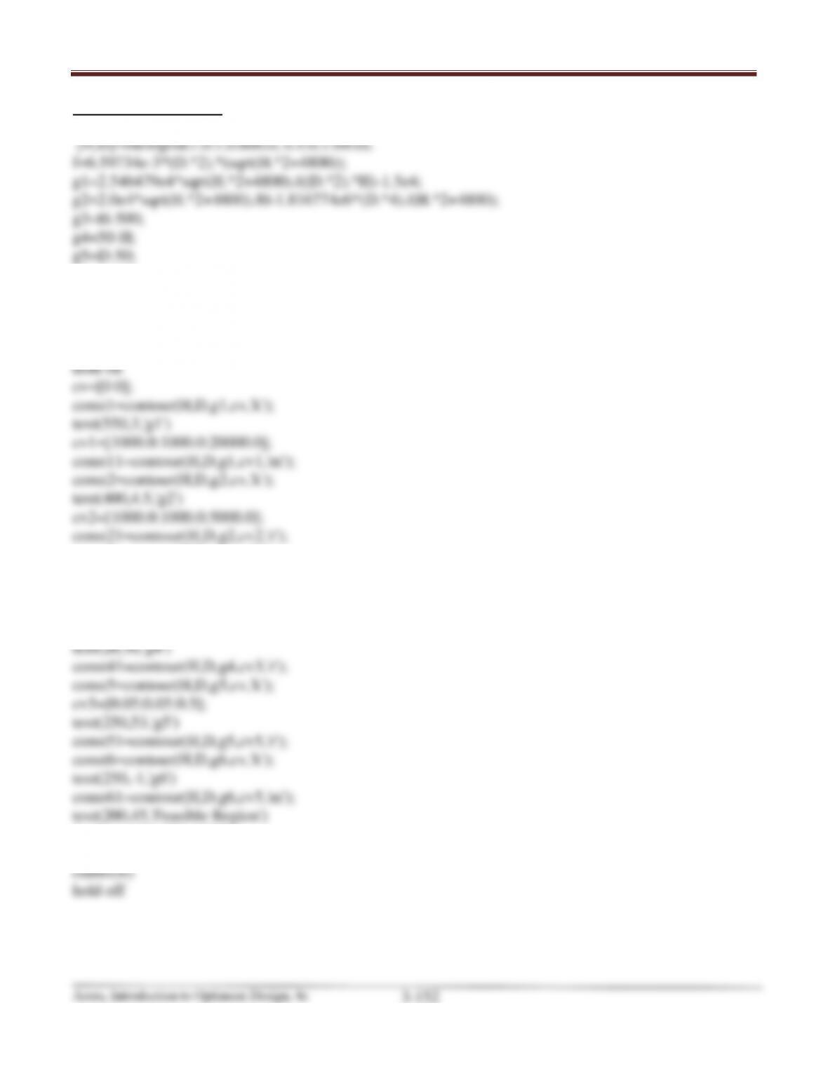
MATLAB Code: 3.54
g6=0.5-D;
cla reset
axis([-20,600,-2,60])
xlabel(‘H‘),ylabel(‘D‘)
title(‘Exercise 3.54′)
const3=contour(H,D,g3,cv,’k’);
cv3=[0.5:0.5:5.0];
text(515,30,’g3′)
const31=contour(H,D,g3,cv3,’r’);
const4=contour(H,D,g4,cv,’k’);
fv=[6.6, 100, 500, 1000];
fs=contour(H,D,f,fv,’k—‘);
Chapter 3 Graphical Solution Method and Basic Optimization Concepts
Alternate formulation
Cost Function: minimize mass;
( )
3f Al
ρ
=
, kg
Constraints:
1
g0
a
P
A
σ
=−≤
cr
2
g= 0
FS
P
P−≤
3
4
5
6
g = 100 0;
g 50 0;
g = 10 0;
g 10
H
H
D
D
−≤
=−+ ≤
−≤
=− +≤
Solution is same as before.
MATLAB CODE FOR ALTERNATE FORMULATION
%Exercise 3.54 – Alternate Formulation
[H,D]=meshgrid(1.0:1.0:120.0, 0.1:0.1:12.0);
%Data for the problem
%Analysis Expressions
L=(H.*H+B.*B./3).^0.5;
I=pi.*D.^4./64;
%Formulation
f=Mass;
Chapter 3 Graphical Solution Method and Basic Optimization Concepts
g6=D_min – D;
cla reset
axis([1,120,.1,12])
cv2=[1000.0:100.0:10000.0];
const21=contour(H,D,g2,cv2,’r’);
const3=contour(H,D,g3,cv,’k’);
cv3=[0.5:0.1:5.0];
text(95,9,’g3′)
const61=contour(H,D,g6,cv5,’m’);
text(60,7,’Feasible Region’)
fv=[4, 6.6, 8, 10, 12];
fs=contour(H,D,f,fv,’k—‘);
clabel(fs)
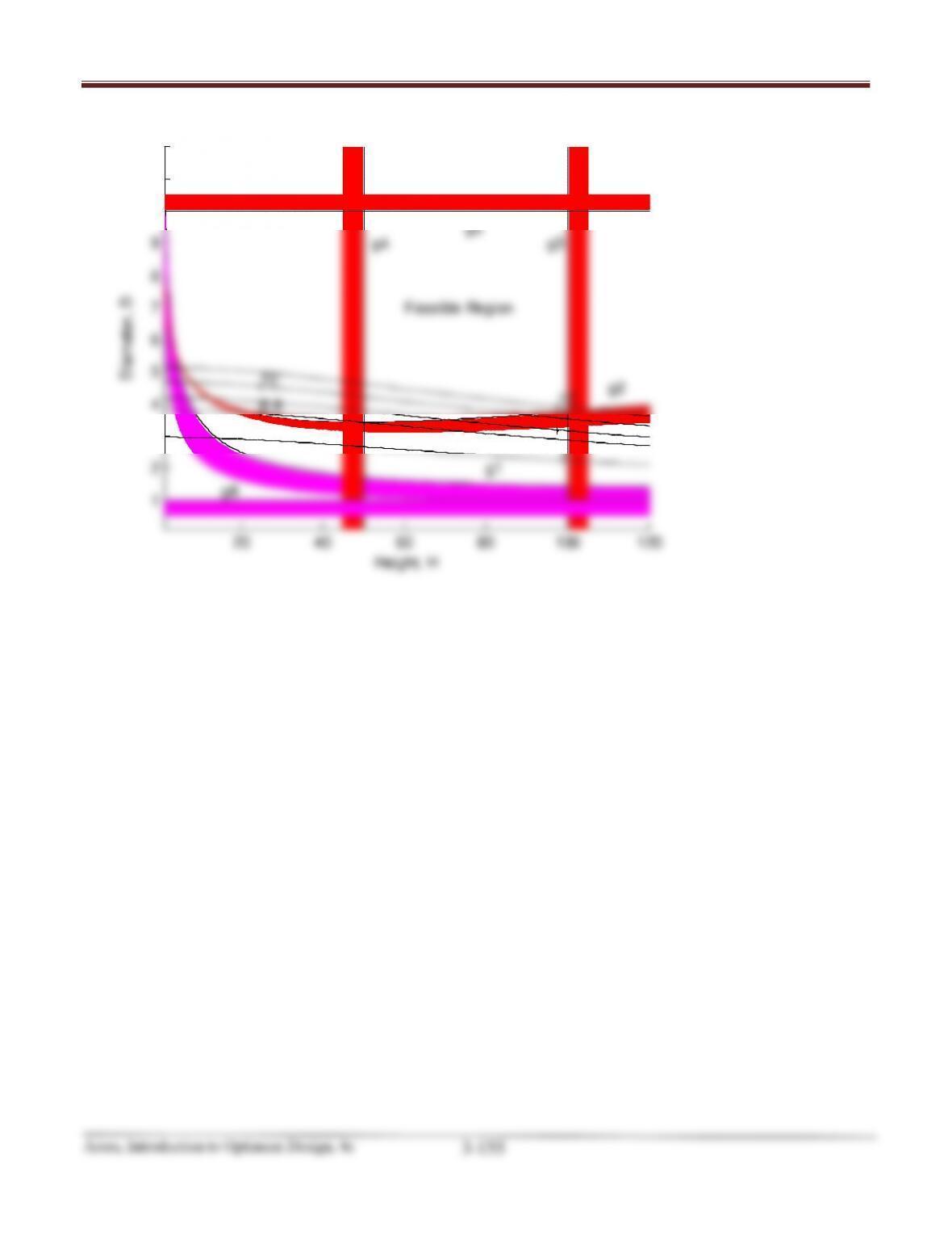
Chapter 3 Graphical Solution Method and Basic Optimization Concepts
20 40 60 80 100 120
1
2
3
4
5
6
7
8
9
10
11
12
Height, H
Diameter, D
Exercise 3.54
g1
g2
g3g4
g5
g6
Feasible Region
4
6.6
8
10
12