Chapter 3 Graphical Solution Method and Basic Optimization Concepts
6
7
g 5000 0;
g 500 0;
A
h
=−≤
= −≤
8
g 3000 0h=−≤
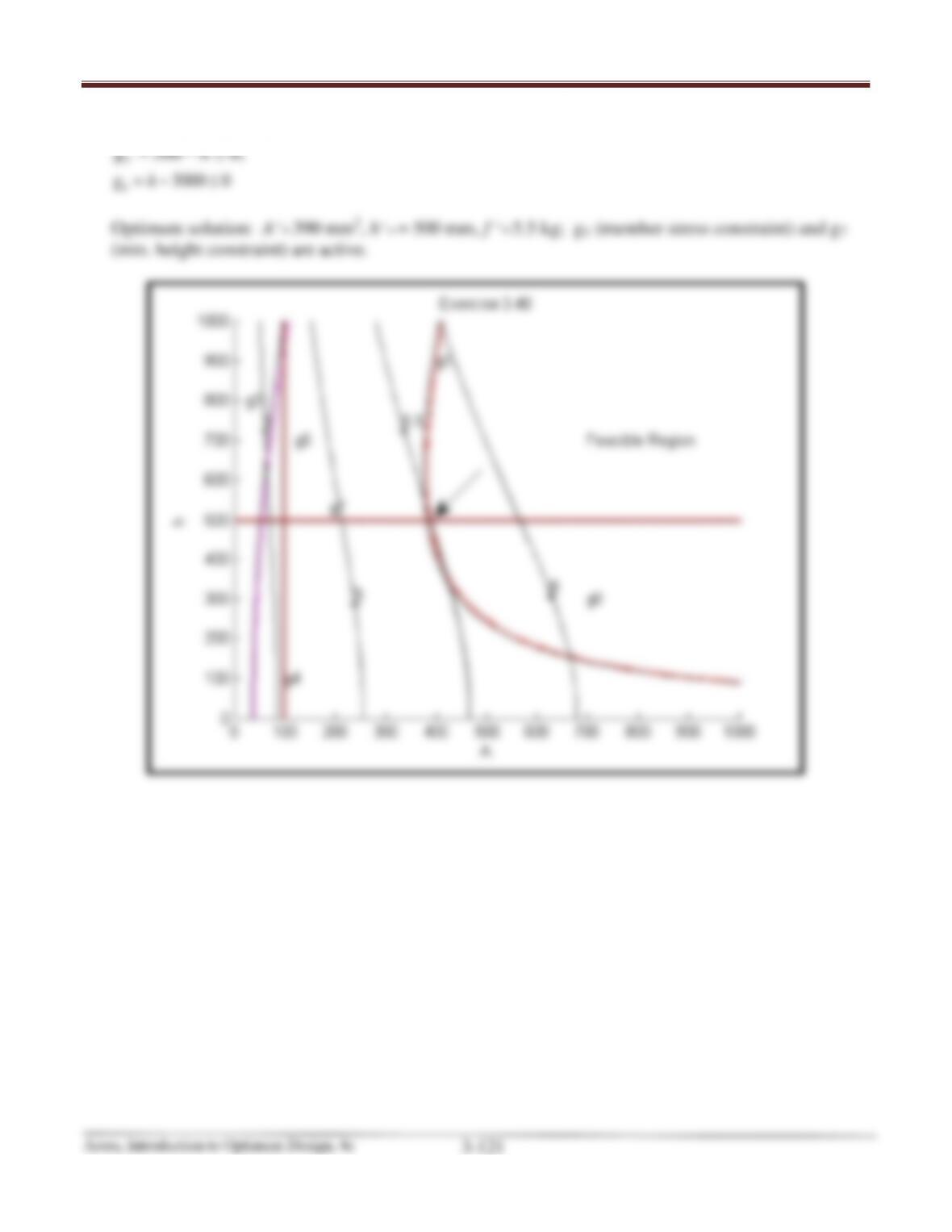
Optimum solution: A
=
∗
390 mm2, h
=
∗
= 500 mm, f
=
∗
5.5 kg; g1 (member stress constraint) and g7
(min. height constraint) are active.
Chapter 3 Graphical Solution Method and Basic Optimization Concepts
MATLAB Code: 3.48
[A,h]=meshgrid(0:10:1000.0, 0:10:1000.0);
ro=7850*1e-9;s=1500;w=10^5;theta=30*pi/180;sa=250;
g6=A–Amax;
g7=-h+hmin;
g8=h–hmax;
cla reset
axis auto %Minimum and maximum values for axes are determined automatically
text(300,1200,’g2′)
cv22=[0.05:0.01: .5];
const21=contour(A,h,g2,cv22,’r’);
cv3=[0 5];
const3=contour(A,h,g3,cv3,’k’);
Chapter 3 Graphical Solution Method and Basic Optimization Concepts
const51=contour(A,h,g5,cv51,’r’);
cv6=[0 5];
const6=contour(A,h,g6,cv1,’k’);
Chapter 3 Graphical Solution Method and Basic Optimization Concepts
Arora, Introduction to Optimum Design, 4e
3-125
8
g 4000 0s=−≤
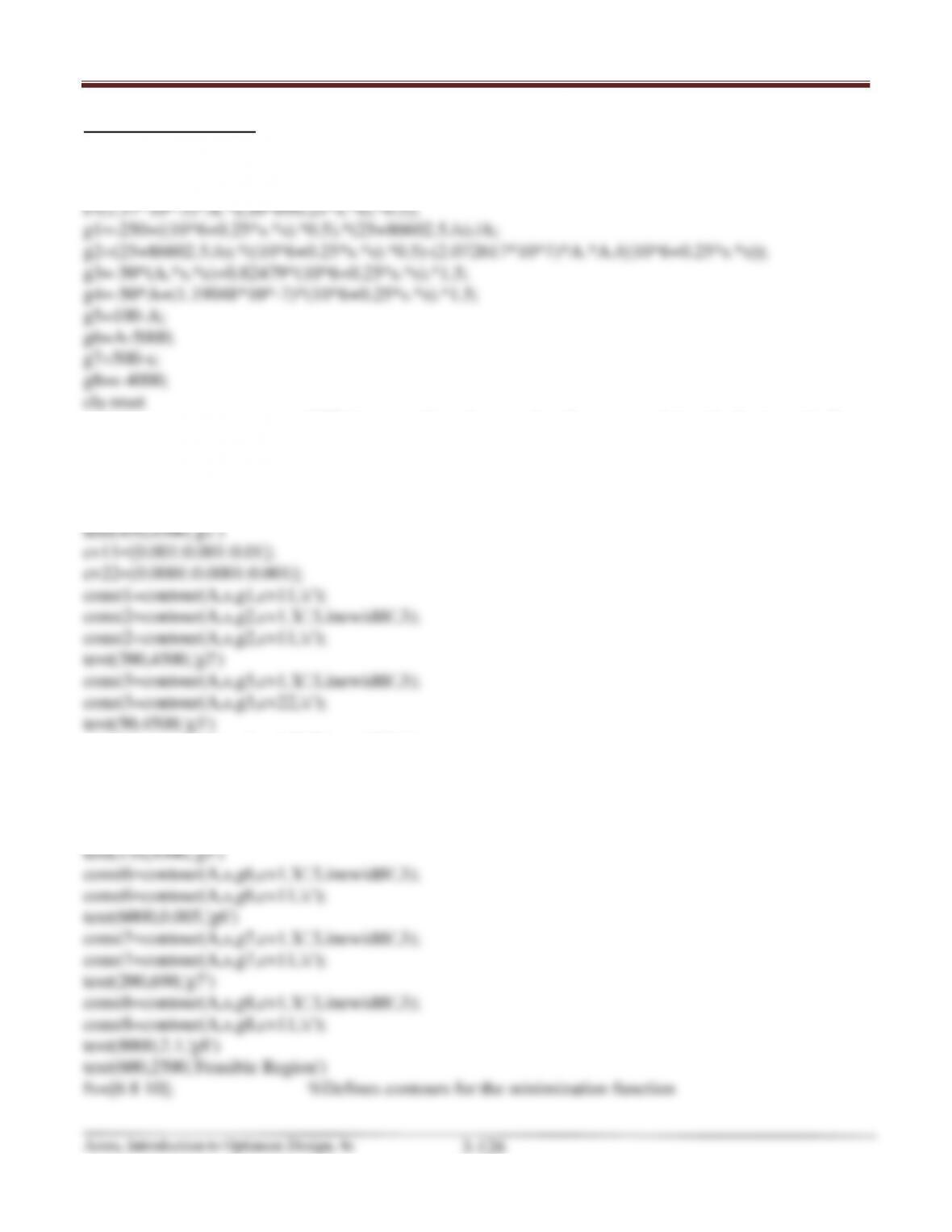
Optimum solution: A
=
∗
410 mm2, s
∗
= 1500 mm, f
=
∗
8.0 kg; g1 (member stress constraint) is active.
Chapter 3 Graphical Solution Method and Basic Optimization Concepts
MATLAB Code: 3.49
[A,s]=meshgrid(0:1:1000, 0:10:5000);
%Enter functions for the minimization problem
axis auto %Minimum and maximum values for axes are determined automatically
xlabel(‘D‘),ylabel(‘H’) %Specifies labels for x– and y-axes
hold on %retains the current plot and axes properties for all subsequent plots
cv1=[0 0];
const1=contour(A,s,g1,cv1,’k’,’LineWidth’,3);
const4=contour(A,s,g4,cv1,’k’,’Linewidth’,4);
const4=contour(A,s,g4,cv11,’c’);
text(25,250,’g4′)
const5=contour(A,s,g5,cv1,’k’,’Linewidth’,3);
const5=contour(A,s,g5,cv11,’c’);
Chapter 3 Graphical Solution Method and Basic Optimization Concepts
fs=contour(A,s,f,fv,’k’); %’k’ specifies black dashed lines for function contours
clabel(fs) %Automatically puts the contour value on the graph
hold off %Indicates end of this plotting sequence
Chapter 3 Graphical Solution Method and Basic Optimization Concepts
3.50 _______________________________________________________________________________
A minimum mass structure (area of member 1 is the same as member 3) three-bar truss is to be
designed to support a load P as shown in Fig. 2.9. The following notation may be used: Pu=P cos,
Pv=P sin, A1 = cross–sectional area of members 1 and 3, A2 = cross–sectional area of member 2.
The members must not fail under the stress, and deflection at node 4 must not exceed 2cm in
either direction. Use Newtons and millimeters as units. The data is given as P = 50 kN; = 30°;
mass density, = 7850 kg/m3; modulus of elasticity, E = 210 GPa; allowable stress, = 150 MPa.
The design variables must also satisfy the constraints 50 ≤Ai ≤5000 mm2 .
Solution
Referring to Section 2.10, the problem is formulated as follows:
6 1 1max
7 2 2 min
8 2 2min
g 0;
g 0;
g0
AA
AA
AA
=−≤
=−+ ≤
=−≤
Use kilogram, Newton and millimeter as units for the given data:
Substituting these data into cost and constraints, we get
( )
( )
( )
( )
( )
( )
( )
63
12 12
1 1 12
2 12
31
4 12
7.85 10 1000 2 2 7.85 10 2 2 ;
g 30618.6 17677.65 2 150 0;
g 35355.3 2 150 0;
g 291.6 20 0;
g 168.4 2 20 0;
f AA AA
A AA
AA
A
AA
−−
=× += × +
= + + −≤
= + −≤
= −≤
= + −≤
Chapter 3 Graphical Solution Method and Basic Optimization Concepts
Arora, Introduction to Optimum Design, 4e
3-129
72
82
g 50 0;
g 5000 0
A
A
=−≤
=−≤
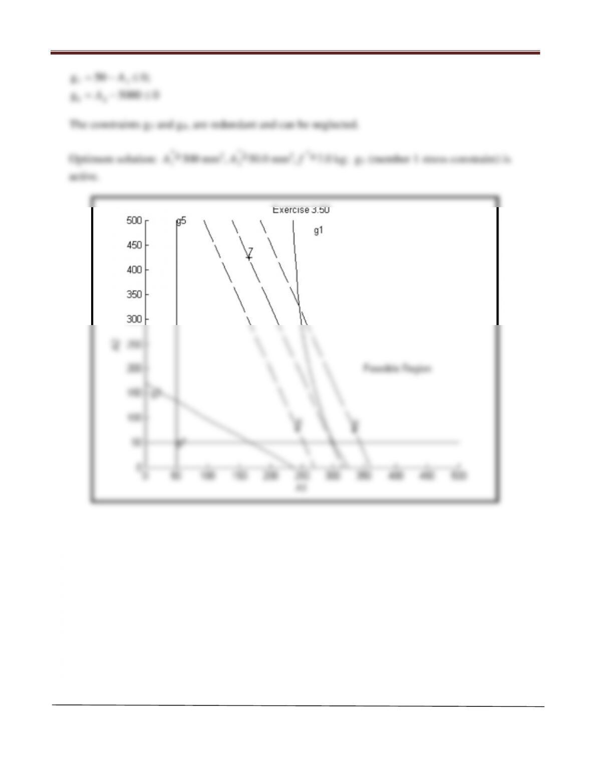
The constraints g3 and g4, are redundant and can be neglected.
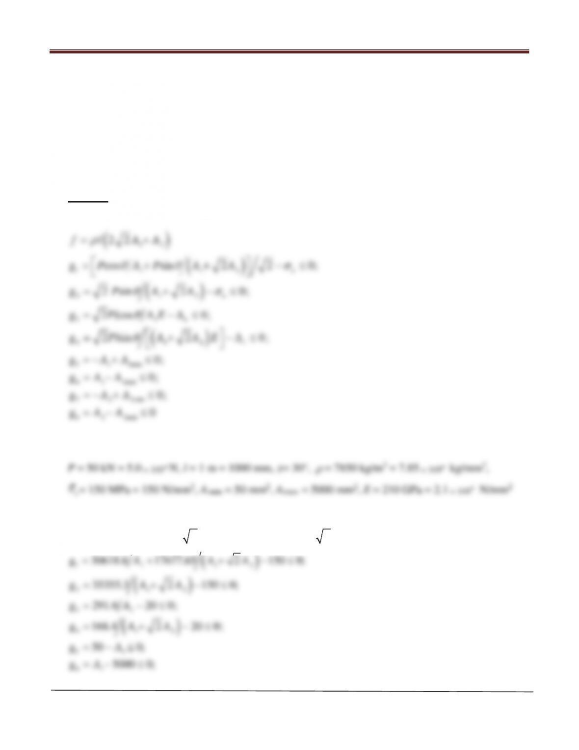
Optimum solution: A
1
∗
=
300 mm2, A
=
∗
2
50.0 mm2, f
=
∗
7.0 kg; g1 (member 1 stress constraint) is
active.
Chapter 3 Graphical Solution Method and Basic Optimization Concepts
MATLAB Code: 3.50
%Create a grid from 0 to 500 with an increment of 1 for the variables A1 and A2
[A1,A2]=meshgrid(0:50:500.0, 0:50:500.0);
axis auto %Minimum and maximum values for axes are determined automatically
%Limits for x– and y–axes may be specified with the command
%axis ([xmin xmax ymin ymax])
xlabel(‘A1‘),ylabel(‘A2‘) %Specifies labels for x– and y-axes
title(‘Exercise 3.50‘)
fv=[6.0, 7.0, 8.0];
fs=contour(A1,A2,f,fv,’k—‘);
Chapter 3 Graphical Solution Method and Basic Optimization Concepts
1=2
12(4+3ℎ)
2=
2(0.5ℎ+)(+ℎ)
Moment at base,
=(+ 0.5ℎ)+(+)
Bending stress,
=
2
Axial stress,
=�
� �=+
(−t)
Combined stress constraint,
+
≤1
Gravitational acceleration,
g = 9.81 m/s2
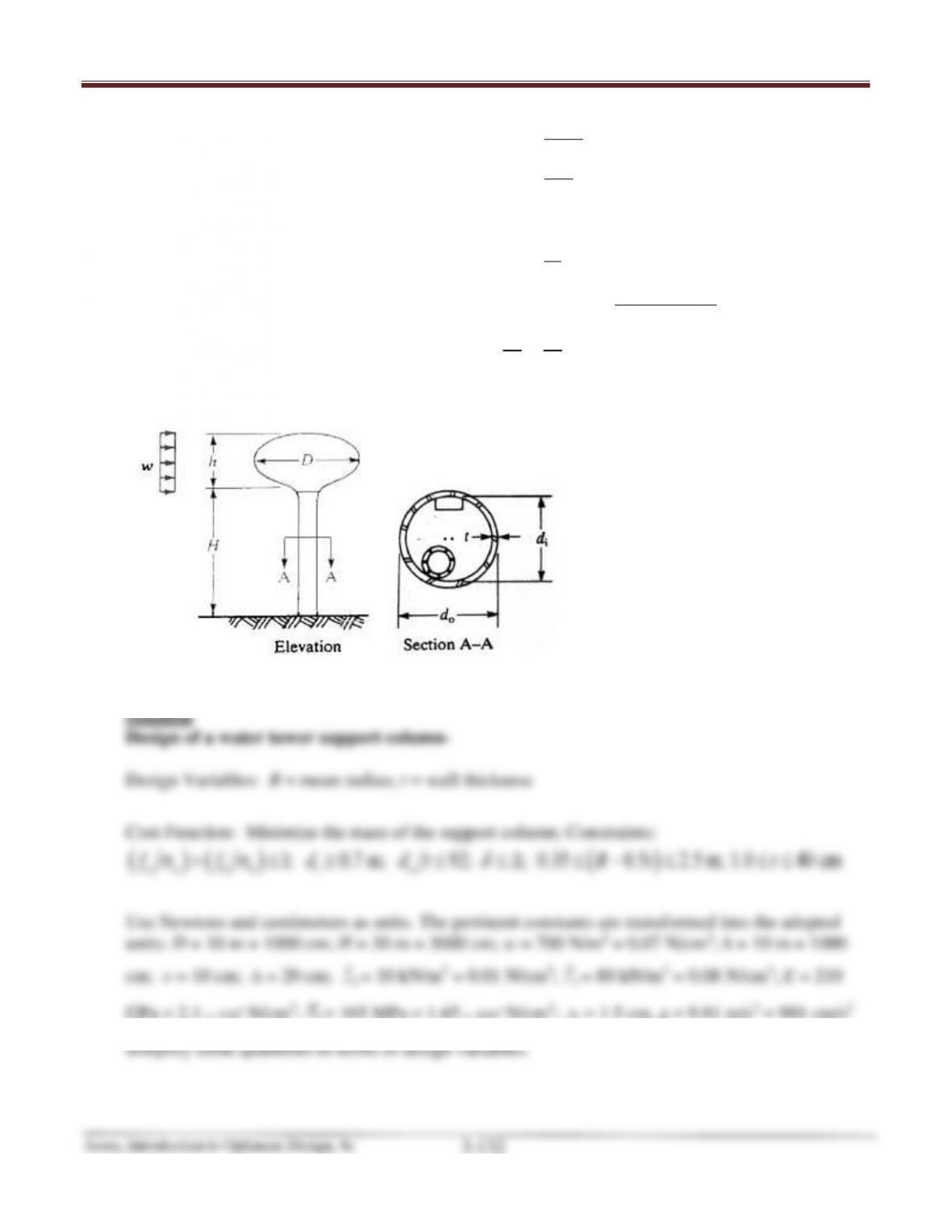
FIGURE E3.51 Water Tower support column.
γ
GPa = 2.1
7
10×
N/cm2;
b
σ
= 165 MPa = 1.65
4
10×
N/cm2; tt = 1.5 cm, g = 9.81 m/s2 = 981 cm/s2
Chapter 3 Graphical Solution Method and Basic Optimization Concepts
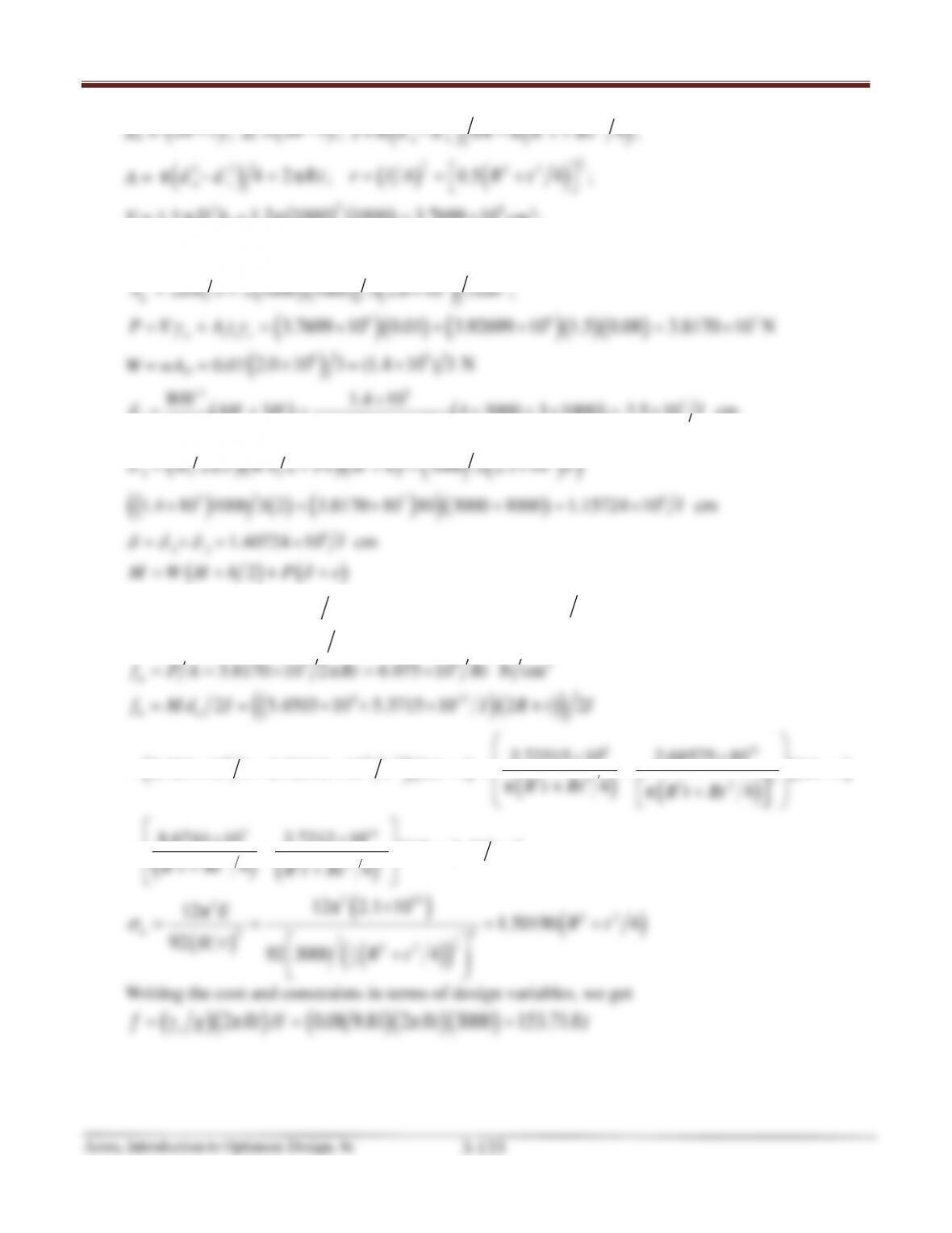
do =
( )
2Rt+
; di =
( )
2Rt−
; I =
( ) ( )
44 3 3
oi
π 64 π 4d d R t Rt−=+
;
A =
( )
( )
( )
1
12
2
2 2 22
oi
π 4 2 π ; 0.5 4 ;d d Rt r I A R t
−= = = +
V = 1.2
( ) ( )
2
29
2
π 1.2π 1000 1000 3.7699 10Dh= = ×
cm3;
( )
262
1.25π 1000 3.92699 10 cm ;
s
A= = ×
( )( )
( )
62
2 3 2 1000 1000 3 2.0 10 3cm ;
p
A Dh= = ×
( )
( )
( )
( )( )
96 7
3.7699 10 0.01 3.92699 10 1.5 0.08 3.8170 10 N
w st s
P V At=+= × + × = ×
γγ
W = wAp = 0.07
( )
65
2.0 10 3 (1.4 10 ) 3 N×=×
( ) ( )
( )
( )
( )( )( )
( )
( )
( )
( )
( )
( )
( )
( ) ( )
( )
( )
25
7
17
7
2
57 8
8
12
5
1.4 10
4 3 4 3000 3 1000 2.5 10 cm
12 3 12 2.1 10
2 2 3000 2 2.1 10
1.4 10 1000 3 2 3.8170 10 10 3000 1000 1.15724 10 cm
1.40724 10 cm
2
1.4 10 3000 500 3 3.81
WH HH I
EI I
H EI W h Pe H h I
I
I
M WH h P e
×
= + = × +× = ×
×
= + += ×
× + × += ×
=+= ×
= +++
=× ++
δ
δ
δδδ
δ
( )( )
78
8 15
70 10 1.40724 10 10
5.45 10 5.3715 10 N cm
I
I
× ×+
= ×+ × ⋅
( )
( )
( )
( )
( )
( ) ( )
( )
7 62
8 15
o
8 15
8 15 2
2
33 33
3.8170 10 2 π 6.075 10 N cm
2 5.4503 10 5.3715 10 2 2
2.72515 10 2.68575 10
2.725 10 2.72515 10 2 2
π4
π4
a
b
f P A Rt Rt
f Md I I R t I
I I Rt Rt
R t Rt R t Rt
==×=×
= = ×+ × +
××
= × + × += + +
+
+
( ) ( )
( )
7 14
2
2
33 33
8.6744 10 2.7212 10 2 N cm
44
Rt
R t Rt R t Rt
××
=++
++
( )
( )
( )
( )
( )
1
2
2 14
2
22
22
22
1
2
12π 2.1 10
12π1.50190 4
92 92 3000 4
a
ERt
Hr Rt
×
= = = +
+
σ
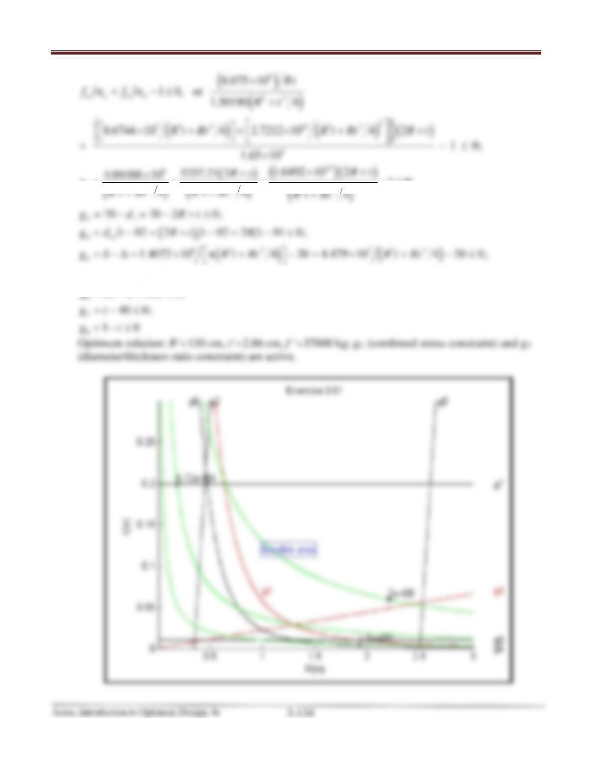
Writing the cost and constraints in terms of design variables, we get
( )( ) ( )( )( )
2 0.08 9.81 2 3000 153.71
s
fgπ Rt H π Rt R t=γ= =
Chapter 3 Graphical Solution Method and Basic Optimization Concepts
( )
( )
( ) ( )
{ }
( )
6
22
2
733 1433
4
6.075 10
1 0, or 1.50190 4
8.6744 10 4 2.7212 10 4 2
1 0;
1.65 10
aa bb
Rt
ff Rt
R t Rt R t Rt R t
×
σ+ σ−≤ +
× + +× + +
+ −≤
×
( )
( )
( ) ( )
( )
( )
( )
( ) ( )
10
6
12
33 33 33
2i
3o
8 33 733
4
5
6
1.6492 10 2
5257.21 2
4.04488 10
g 1 0;
44 4
g 70 70 2 0;
g 92 2 92 2 91 0;
gΔ 1.4072 10 π 4 20 4.479 10 4 20 0;
g 0.5 250 0 ;
g
Rt
Rt
R t Rt R t Rt R t Rt
d Rt
d t R t t Rt
R t Rt R t Rt
Rt
×+
+
×
= + + −≤
++ +
= − = − +≤
= −= + −= −≤
=δ− = × + − = × + − ≤
=−−≤
7
8
35 0.5 0;
g 40 0;
g1 0
Rt
t
t
= −+ ≤
=−≤
=−≤
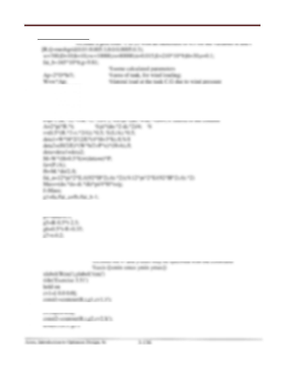
Optimum solution: R
=
∗
130 cm, t
=
∗
2.86 cm, f
=
∗
57000 kg; g1 (combined stress constraint) and g3
(diameter/thickness ratio constraint) are active.

Chapter 3 Graphical Solution Method and Basic Optimization Concepts
Arora, Introduction to Optimum Design, 4e
3-135
Chapter 3 Graphical Solution Method and Basic Optimization Concepts
MATLAB Code: 3.51
V=1.2*pi*D^2*h;
As=1.25*pi*D^2;
P=V*rw+As*tt*rs;
do=2*R+t; % diameter of outside column
di=2*R-t; % diameter of inside column
g2=0.7-di;
g3=do./t-92;
g8=0.01-t;
cla reset
axis auto %Minimum and maximum values for axes are determined automatically
text(1.0,0.07,’g1′,’color’,’r’)
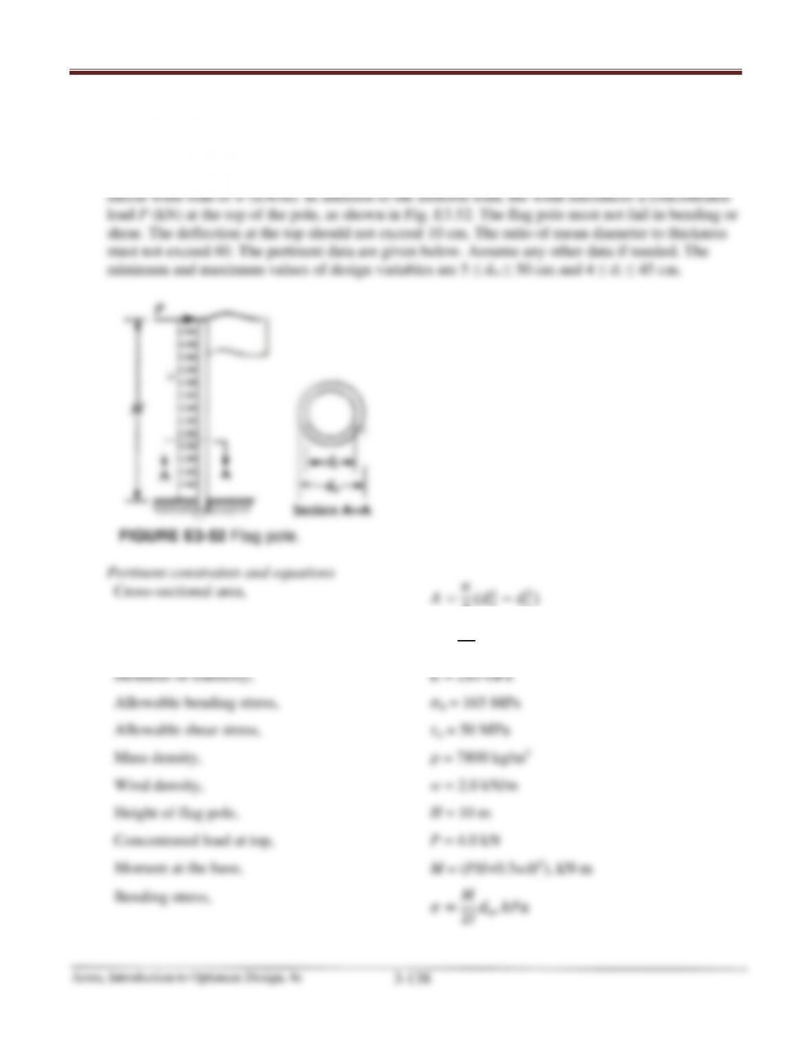
Chapter 3 Graphical Solution Method and Basic Optimization Concepts
3.52*___________________________________________________________________________
Design of a flag pole. Your consulting firm has been design a minimum mass flag pole of height
H. The pole will be made of uniform hollow circular tubing with do and di as outer and inner
diameters, respectively. The pole must not fail under the action of high winds.
For design purpose, the pole will be treated as a cantilever that is subjected to a uniform