Chapter 3 Graphical Solution Method and Basic Optimization Concepts
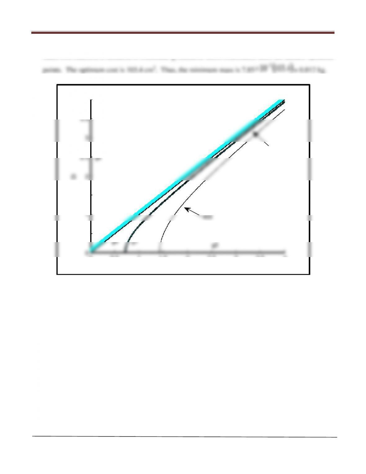
Since cost function is identical to constraint
1
g
(member stress constraint), there are infinite optimum
3
−
00.5 11.5 22.5 33.5 4
0
0.5
1
1.5
2
2.5
3
3.5
4
Do
Di
g1
g2
g3
g4
Exercise 3.26
400
103.4
Chapter 3 Graphical Solution Method and Basic Optimization Concepts
MATLAB Code
[Do,Di]=meshgrid(0:0.01:4, 0:0.01:4);
%Enter functions for the minimization problem
g1=13.1675-25*(Do.^2-Di.^2);
g2=–Do;
g3=–Di;
text(0.85,0.3,’g1′)
cv11=[0.01:0.01:0.1];
text(0.1,2.5,’g2′)
text(2.5,0.2,’g3′)
text(0.45,0.3,’g4′)
text(120,20,’Feasible Region’)
fv=[103.4 400]; %Defines contours for the minimization function
fs=contour(Do,Di,f,fv,’k’); %’k’ specifies black dashed lines for function contours
Chapter 3 Graphical Solution Method and Basic Optimization Concepts
MATLAB Code
[A,h]=meshgrid(3000:5:5500, 10:0.1:22);
%Enter functions for the minimization problem
f=0.6*h+0.001*A;
g1=20000*3.5-h.*A;
g2=0.25*h.*A+A*3.5-10000*3.5;
g3=3.5-h;
g4=h-21;
g5=–A;
cla reset
text(2.5,0.2,’g3′)
const4=contour(A,h,g4,cv1,’k’,’Linewidth’,4);
fv=[13.4 15 16]; %Defines contours for the minimization function
fs=contour(A,h,f,fv,’k’); %’k’ specifies black dashed lines for function contours
Chapter 3 Graphical Solution Method and Basic Optimization Concepts
Arora, Introduction to Optimum Design, 4e
3-66
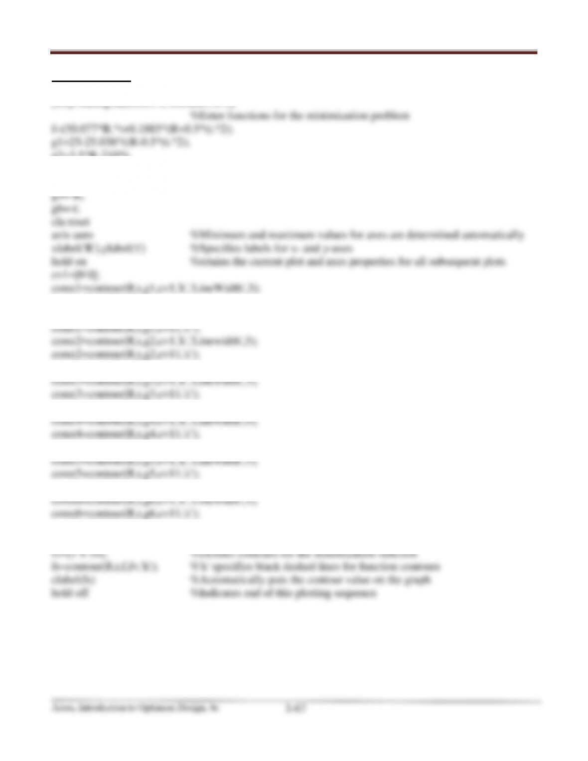
Mean radius should be greater than t/2:
Both R and t should be greater than zero:
5
6
g 0,
g0
R
t
=−≤
=−≤
∗
∗
00.5 11.5 22.5 33.5 4
0
0.01
0.02
0.03
0.04
0.05
0.06
0.07
0.08
0.09
0.1
R
t
g1
g2
g3
g4
g5
g6
Feasible Region
1
6
10
Exercise 3.28
Chapter 3 Graphical Solution Method and Basic Optimization Concepts
MATLAB Code.
[R,t]=meshgrid(0:0.01:4, 0:0.0001:0.1);
g2=3.5*R-210*t;
g3=(1.41667*10^-5)*R-0.001*t;
g4=-R+0.5*t;
text(1.15,0.07,’g1′)
cv11=[0.01:0.01:0.1];
text(2.5,0.0475,’g2′)
text(2.5,0.03,’g3′)
text(0.1,0.06,’g4′)
text(0.1,0.02,’g5′)
text(2.5,0.005,’g6′)
text(2,0.07,’Feasible Region’)
Chapter 3 Graphical Solution Method and Basic Optimization Concepts
Arora, Introduction to Optimum Design, 4e
3-69
( )
45
5 11 2
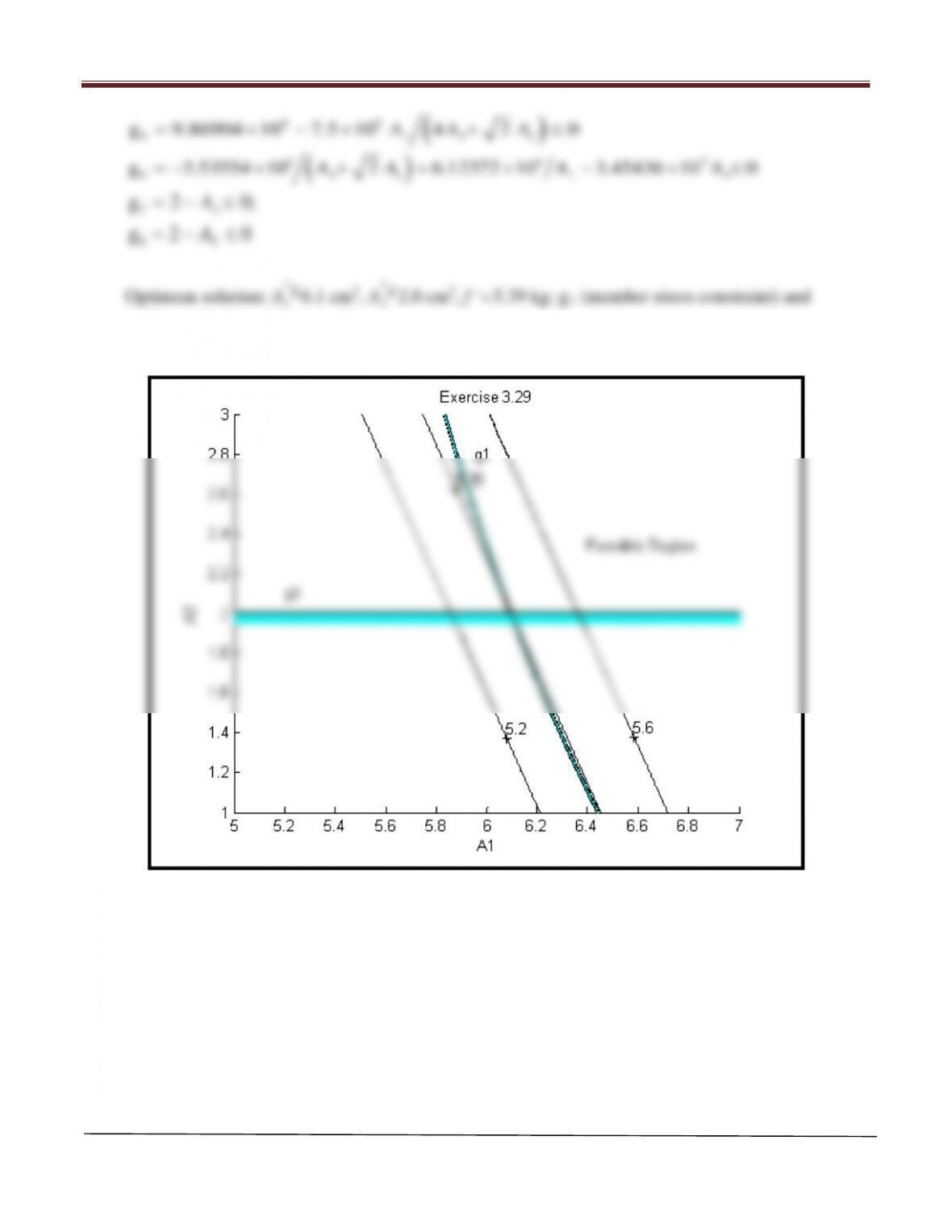
g 9.86904 10 7.5 10 4 2 0AA A= × −× + ≤
( )
4 43
6 12 1 1
g 3.53554 10 2 6.12372 10 3.45436 10 0AA A A=− × + + × − ×≤
71
82
g 2 0;
g2 0
A
A
=−≤
=−≤
∗
∗
∗
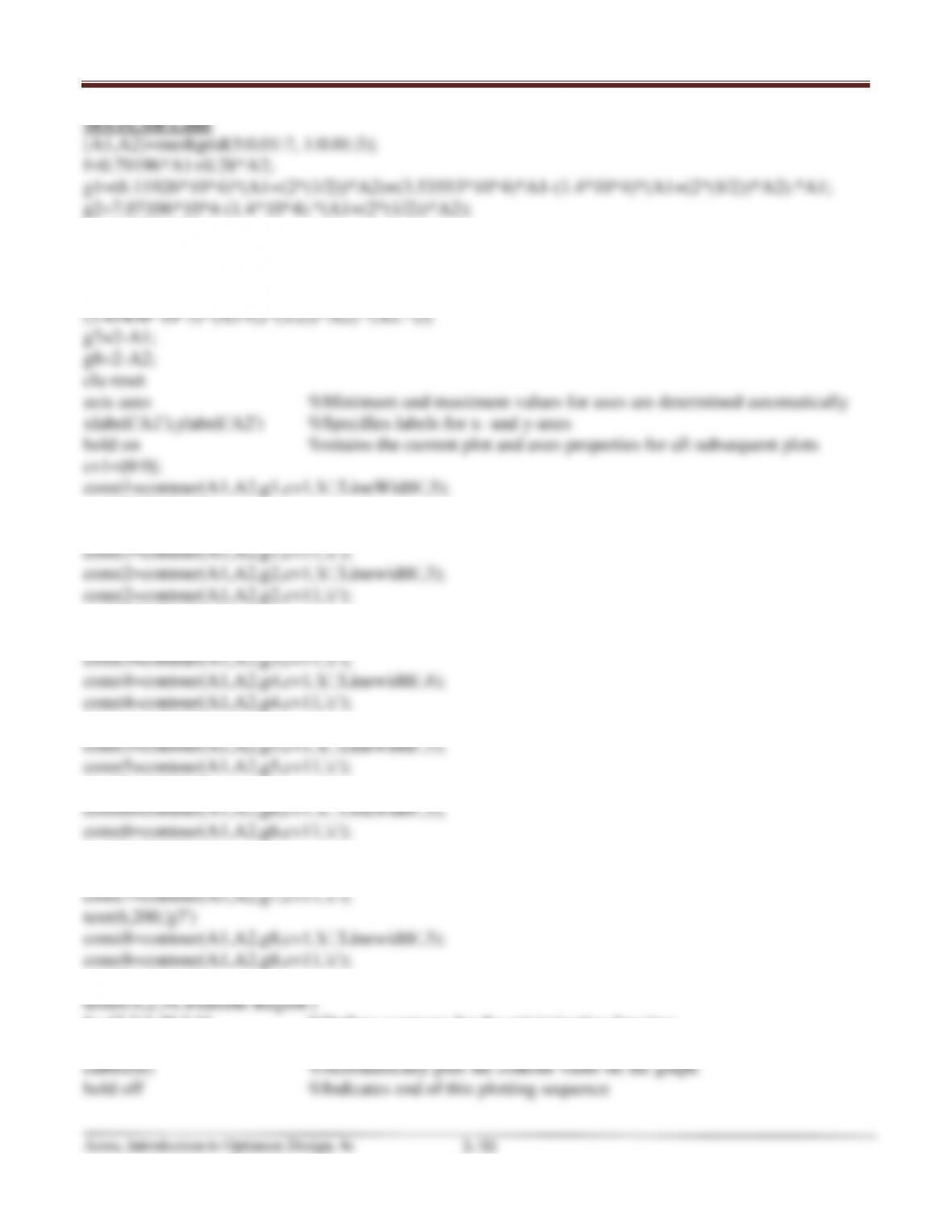
g8 (lower limit on A2) are active.
Chapter 3 Graphical Solution Method and Basic Optimization Concepts
MATLAB Code
[A1,A2]=meshgrid(5:0.01:7, 1:0.01:3);
f=0.79196*A1+0.28*A2;
g1=(6.11926*10^4)*(A1+(2^(1/2))*A2)+(3.53553*10^4)*A1-(1.4*10^4)*(A1+(2^(1/2))*A2).*A1;
g2=7.07106*10^4-(1.4*10^4).*(A1+(2^(1/2))*A2);
g3=1.7496-0.5*A1;
g4=1.01016-0.5.*(A1+(2^(1/2))*A2);
g5=(9.86904*10^4)*(4*A1+(2^(1/2))*A2)-(7.5*10^5)*A1;
g6=(6.12372*10^4)*(A1+(2^(1/2))*A2)-(3.53553*10^4)*A1-
text(5.95,2.8,’g1′)
cv11=[0.01:0.001:0.05];
text(2.5,0.0475,’g2′)
const3=contour(A1,A2,g3,cv1,’k’,’Linewidth’,3);
text(0.1,0.06,’g4′)
text(0.1,0.02,’g5′)
text(2.5,0.005,’g6′)
const7=contour(A1,A2,g7,cv1,’k’,’Linewidth’,3);
text(5.2,2.1,’g8′)
fv=[5.2 5.39 5.6]; %Defines contours for the minimization function
fs=contour(A1,A2,f,fv,’k’); %’k‘ specifies black dashed lines for function contours
Chapter 3 Graphical Solution Method and Basic Optimization Concepts
3.30 ________________________________________________________________________________
Consider the cabinet design problem given in Section 2.6. Use the equality constraints to eliminate
three design variables from the problem. Restate the problem in terms of the remaining three
variables, transcribing it into the standard form.
Solution
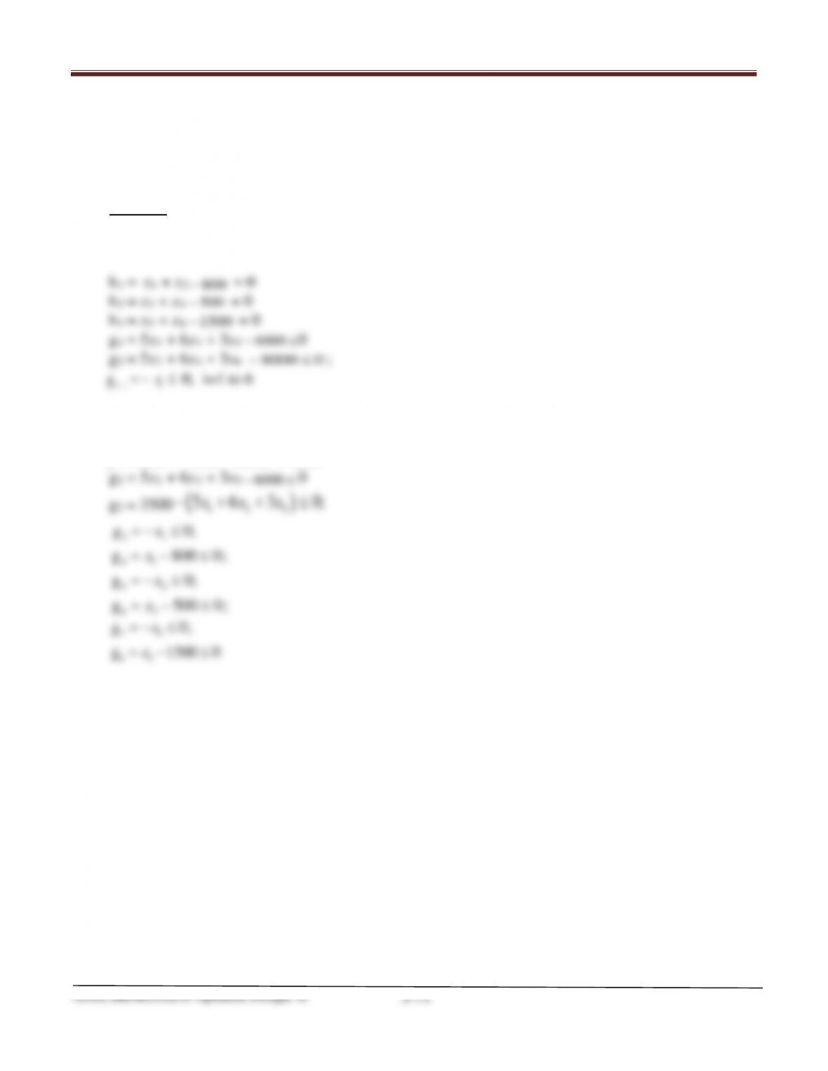
f = 3.5x1 + 3.0x2 + 6.0x3 + 4.8x4 + 1.8x5 + 3.0x6
Using the three equality constraints to eliminate x2, x4 and x6 from all the other equations, we get
f = 0.5x1 + 1.2x3
21.−
x5 + 9300
Arora, Introduction to Optimum Design, 4e
3-73
3.32________________________________________________________________________________
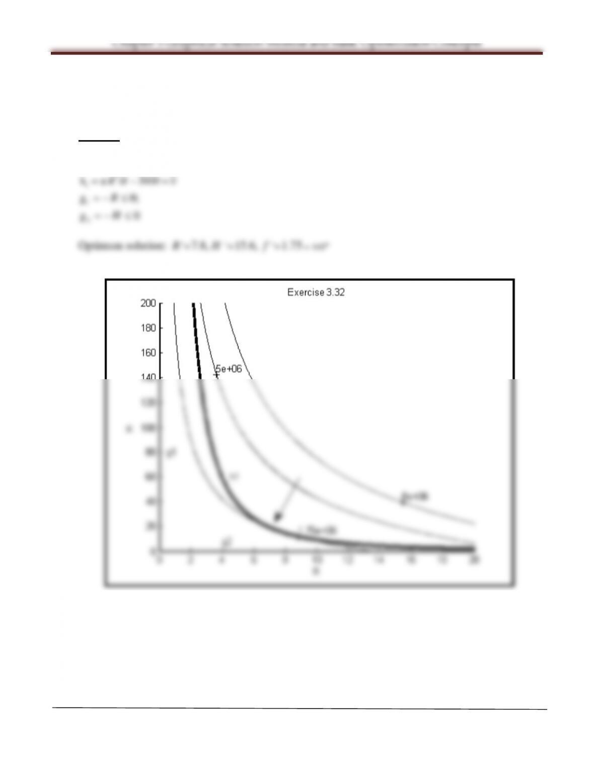
Solve the cylindrical tank design problem given in Section 2.8 graphically for the following data:
c=$1500/m2, V=3000 m3.
Solution
f =1500(
2
2π 2πR RH+
);
2
1
hπ 3000 0RH= −=
1
2
g 0;
g0
R
H
=−≤
=−≤
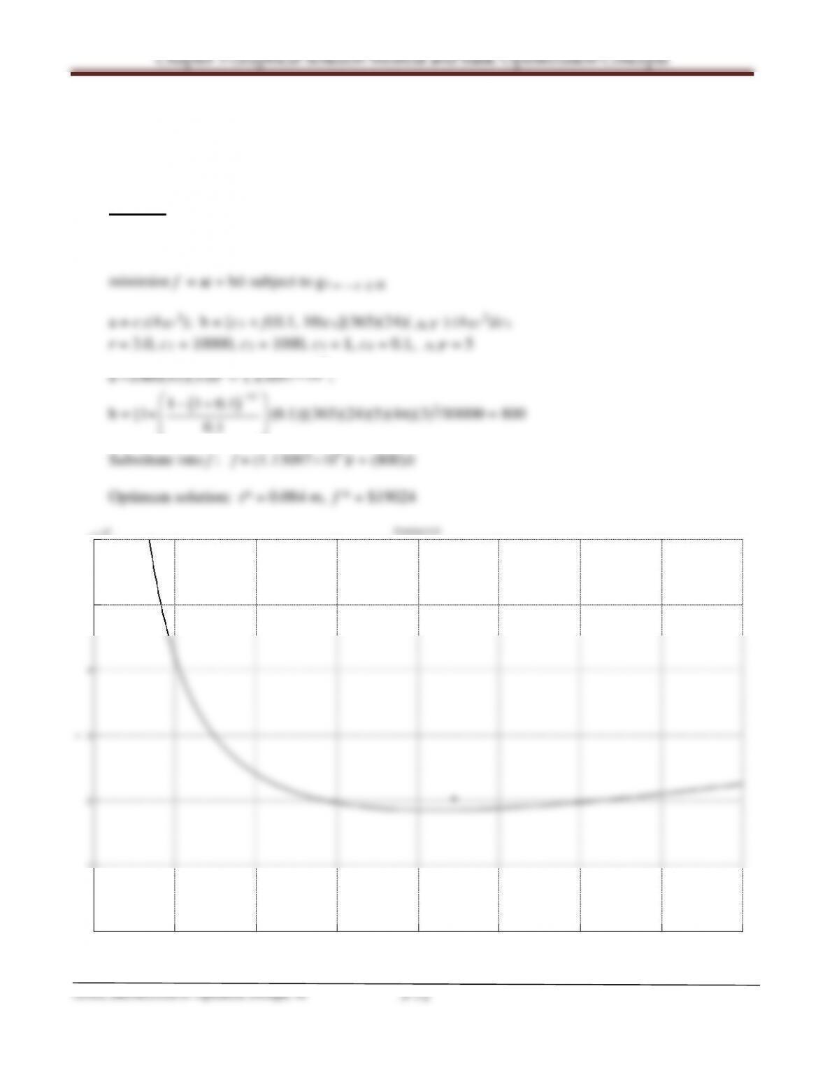
Optimum solution: R
=
∗
7.8, H
=
∗
15.6, f
=
∗
1.75
6
10×
Chapter 3 Graphical Solution Method and Basic Optimization Concepts
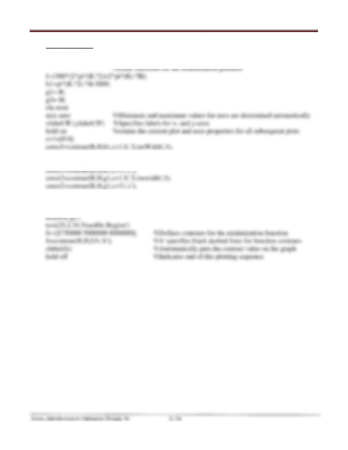
MATLAB Code
[R,H]=meshgrid(0:0.1:20, 0:1:200);
text(4.5,60,’h1′)
cv11=[0.01:0:0.01];
text(0.5,80,’g1′)
const3=contour(R,H,g2,cv1,’k’,’Linewidth’,3);
const3=contour(R,H,g2,cv11,’c’);
Chapter 3 Graphical Solution Method and Basic Optimization Concepts
3.33________________________________________________________________________________
Consider the minimum mass tubular column problem formulated in Section 2.7. Find the optimum
solution for the problem using the graphical method for the data:
load, P = 100 kN; length, l = 5.0 m; Young’s modulus, E = 210GPa; allowable stress, = 250
MPa; mass density, =7850 kg/m3, R ≤ 0.4 m; t ≤ 0.1 m; R, t ≥ 0.
Solution
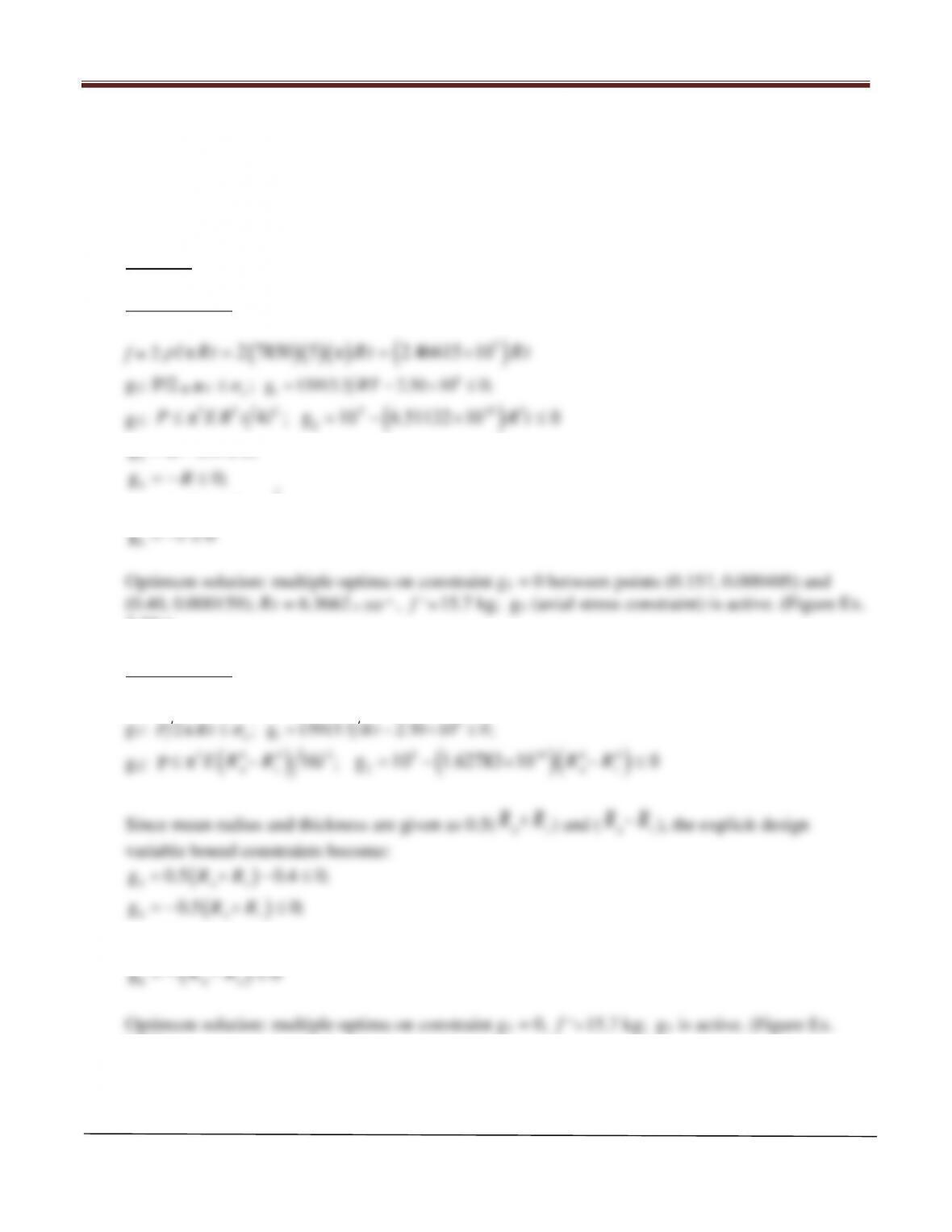
Formulation 1: Design Variables: R = mean radius of the column; t = wall thickness
5
Chapter 3 Graphical Solution Method and Basic Optimization Concepts
Arora, Introduction to Optimum Design, 4e
3-76
Chapter 3 Graphical Solution Method and Basic Optimization Concepts
MATLAB Code
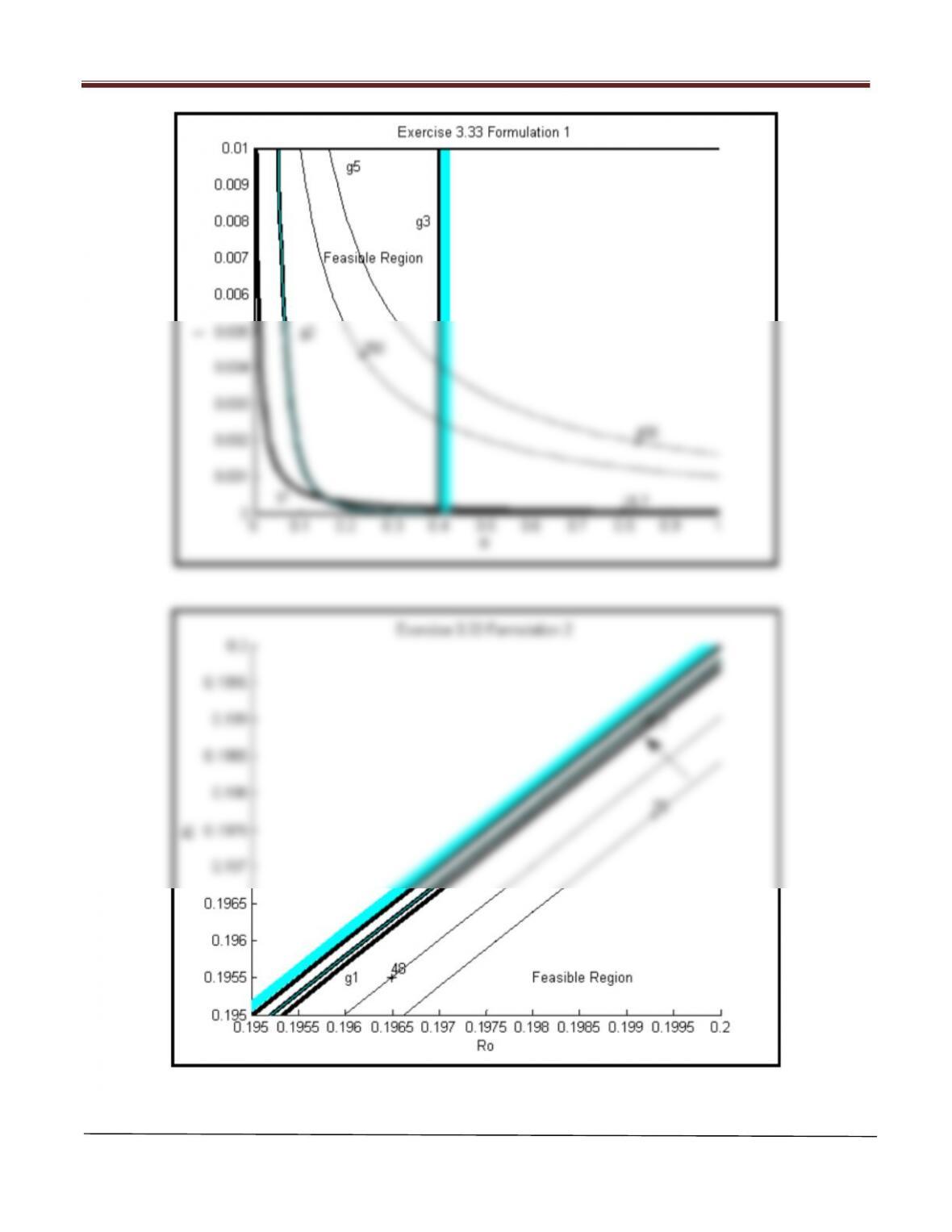
Formulation 1:
[R,t]=meshgrid(0:0.01:1, 0:0.001:0.01);
%Enter functions for the minimization problem
f=(2.46615*10^5)*R.*t;
g1=15915.5-(2.50*10^8)*R.*t;
g2=10^5-(6.51132*10^10)*(R.^3).*t;
g3=R-0.4;
text(0.05,0.0005,’g1′)
cv11=[0.001:0.001:0.02];
text(0.1,0.005,’g2′)
text(0.35,0.008,’g3′)
const4=contour(R,t,g4,cv1,’k’,’Linewidth’,3);
text(0.2,0.0095,’g5′)
fv=[15.7 250 400]; %Defines contours for the minimization function
fs=contour(R,t,f,fv,’k’); %’k’ specifies black dashed lines for function contours
Chapter 3 Graphical Solution Method and Basic Optimization Concepts
MATLAB Code
Formulation 2:
[Ro,Ri]=meshgrid(0.195:0.001:0.2, 0.195:0.001:0.2);
%Enter functions for the minimization problem
cla reset
axis auto %Minimum and maximum values for axes are determined automatically
xlabel(‘Ro’),ylabel(‘Ri’) %Specifies labels for x– and y–axes
hold on %retains the current plot and axes properties for all subsequent plots
cv1=[0 0];
const1=contour(Ro,Ri,g1,cv1,’k’,’LineWidth’,3);
text(0.196,0.1955,’g1′)
cv11=[0.00005:0.00001:0.0002];
text(0.1,0.005,’g2′)
text(0.35,0.008,’g3′)
const4=contour(Ro,Ri,g4,cv1,’k’,’Linewidth’,3);
text(0.2,0.0095,’g5′)
text(0.198,0.1955,’Feasible Region’)
fv=[15.7 48 78]; %Defines contours for the minimization function
fs=contour(Ro,Ri,f,fv,’k’); %’k’ specifies black dashed lines for function contours
Chapter 3 Graphical Solution Method and Basic Optimization Concepts
Arora, Introduction to Optimum Design, 4e
3-80
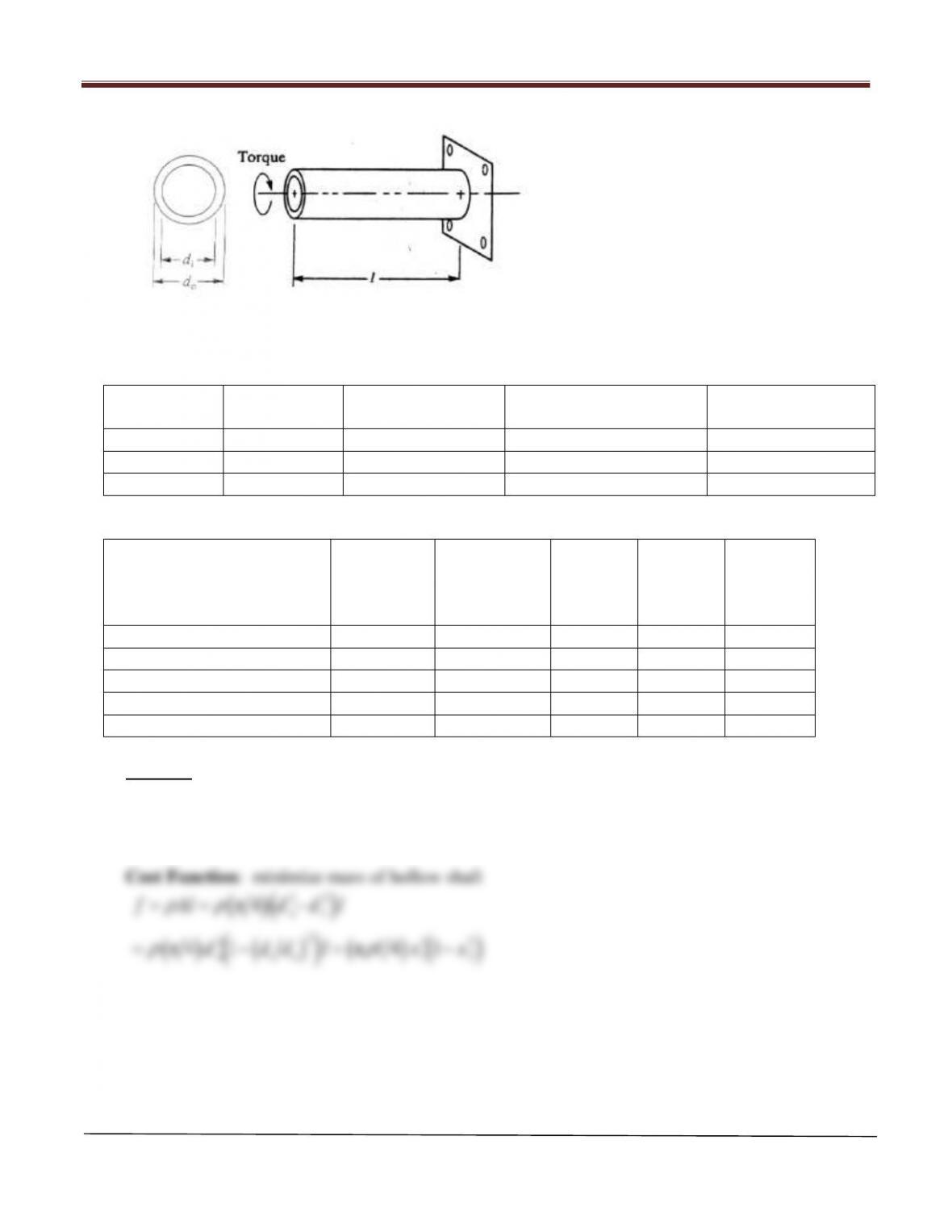
FIGURE E3–34 Hollow torsion rod.
TABLE E3–34(A) Rod Requirements
Torsion rod
number
Length,
l (m)
Normal torque,
T0 (kN
⋅
m)
Max. torque,
Tmax (kN
⋅
m)
Allowable twist,
(degrees)
1
0.50
10.0
20.0
2
2
0.75
15.0
25.0
2
3
1.00
20.0
30.0
2
TABLE E3–34(B) Materials and Properties for the Torsion Rod
Material
Density,
(kg/m3),
Allowable
Shear stress,
(MPa)
Elastic
modulus,
E (GPa)
Shear
modulus,
G (GPa)
Poisson’s
ratio (
)
1. 4140 alloy steel
7850
275
210
80
0.30
2. Aluminum alloy 24 ST4
2750
165
75
28
0.32
3. Magnesium alloy A261
1800
90
45
16
0.35
4. Berylium
1850
110
300
147
0.02
5. Titanium
4500
165
110
42
0.30
Solution
Design Variables: x1 = outside diameter of the shaft; x2 = ratio of inside/outside diameter, di/do
Units of mass, force and length are kg, N and mm respectively.
( ) ( )
( )
( )
( )
2 22
o io 1 2
π4 1 π 4 1
d dd l l x x
ρρ
= −= −
Constraints: